Try the code yourself!

Click the following button to launch an ipython notebook on Google Colab which implements the code developed in this post:

The Problem

Have you ever wondered if you could calculate $\pi$ by simply dropping toothpicks on the floor? In the 18th century, French mathematician Georges-Louis Leclerc, Comte de Buffon, wondered exactly that. Not with toothpicks specifically but using needles. However the principle remains the same, and it results in an interesting demonstration of how probability and geometry can intertwine.

Imagine you have a floor made of parallel wooden floorboards, each of equal width. If you drop a toothpick on this floor, what is the probability that the toothpick will cross one of the lines between the floorboards? How can we use this to calculate $\pi$?

In this post we are going to answer this question.

The Mathematics

We have parallel floorboards of width $d$
We drop a toothpick of length $l$ (where $l \le d$)
We want to know the probability, $P$, that the toothpick crosses a line, the separation between two floorboards

Buffon proved that this probability equals

\[P = \frac{2l}{\pi d}\]

Note how $\pi$ appears in this formula. Rearranging this equation to solve for $\pi$ gives

\[\pi = \frac{2l}{P d}\]

This means we can estimate $\pi$ by:

Dropping lots of toothpicks
Counting how many cross between two floorboards
Plugging that empirical probability into this formula

The more toothpicks we drop, the closer our estimate should get to the true value of $\pi$. This is one of the earliest examples of a Monte Carlo method using random sampling to obtain numerical results.

For those that want to see the full derivation, see the section at the end of this post.

Buffon first proposed this problem in 1733, but published the solution in 1777, and I would consider it one of oldest problems in geometric probability, preceding much of the formal development of probability theory.

Simulating the Experiment with Python

Rather than dropping thousands of actual toothpicks (and spending hours cleaning them up), let’s use Python to simulate the experiment.

We are going to create a function in order to run a Buffon needle simulation and we will break down the code section by section. Here is a rough thought process for what we are aiming to do:

Let’s break down how our simulation works:

Setting Up the Experiment: We define the distance between lines and the length of our toothpicks.
Random Needle Drops: For each toothpick, we randomly determine:
- Its position (x, y coordinates)
- Its angle $\theta$ relative to the parallel lines
Detecting Crossings: A toothpick crosses a line if its endpoints are on opposite sides of any line.
Calculating $\pi$: We apply Buffon’s formula to estimate $\pi$ based on the proportion of toothpicks that cross lines.
Visualization: We create plots showing both the physical experiment (toothpicks on lines) and how our estimate of $\pi$ converges as we drop more toothpicks.

1. Imports and Setup

import numpy as np
import matplotlib.pyplot as plt
from matplotlib.animation import FuncAnimation
from matplotlib.lines import Line2D
import matplotlib.gridspec as gridspec
from typing import List, Tuple, Optional

numpy provides numerical computation functions
matplotlib.pyplot handles plotting and visualization
FuncAnimation creates animations from matplotlib plots
Line2D is used to create legend elements
gridspec allows for complex subplot grid layouts
typing provides type hints for better code clarity

2. Needle Simulation Function

def simulate_buffon_needle_batch(
    batch_size: int, 
    needle_length: float = 1, 
    line_distance: float = 1, 
    floor_width: float = 10
) -> Tuple[int, List[Tuple[float, float, float]]]:

This function simulates dropping a batch of needles onto the floor and counts how many cross lines.

    # generate random positions and angles for needles
    x_positions = np.random.uniform(0, floor_width, batch_size)
    thetas = np.random.uniform(0, np.pi, batch_size)
    y_positions = np.random.uniform(0, 10, batch_size)

creates random x-positions across the floor width
creates random angles between 0 and $\pi$ radians
creates random y-positions for visualization (between 0 and 10)

    # for calculation: find distance to nearest line
    nearest_line_positions = np.floor(x_positions / line_distance) * line_distance
    distances_to_nearest_line = x_positions - nearest_line_positions

calculates the position of the nearest line to the left of each needle
calculates how far each needle is from its nearest line

    # determine which needles cross a line
    needle_half_length = needle_length / 2
    
    crossing_left = distances_to_nearest_line < needle_half_length * np.sin(thetas)
    crossing_right = distances_to_nearest_line > line_distance - needle_half_length * np.sin(thetas)
    crossings = np.sum(crossing_left | crossing_right)

a needle crosses a line if its distance to the nearest line is less than $(L/2)\sin\theta$
or if its distance to the next line to the right is less than $(L/2)\sin\theta$
the total number of crossings is counted

    # prepare needle data for visualization
    needles = [(x_positions[i], y_positions[i], thetas[i]) for i in range(batch_size)]
    
    return crossings, needles

packages the needle position and angle data for visualization
returns both the crossing count and needle data

3. Animation Creation Function

def create_buffon_animation(
    total_needles: int = 1000,
    batch_size: int = 10,
    needle_length: float = 0.8,
    line_distance: float = 1.0,
    floor_width: float = 10.0,
    fps: int = 30,
    duration: int = 20,
    output_file: str = 'buffon_needle_animation.mp4'
):

This function creates the animation by dropping needles in batches and updating the visualization.

    # helper function to format the error text with color
    def error_color_text(error_percent, color):
        """Format the error text with color."""
        
        return f'$\\color{{{color}}}{{{error_percent:.4f}\\%}}$'
        

a nested helper function that creates colored text for the error display
uses LaTeX formatting so the color can be displayed in matplotlib

    # calculate frames needed
    frames = min(total_needles // batch_size, fps * duration)

determines how many animation frames to create
limits it to either the total number of needle batches or the maximum frames for the duration

    # set up the figure with two subplots
    fig = plt.figure(figsize=(12, 8))
    gs = gridspec.GridSpec(2, 1, height_ratios=[2, 1])

creates a figure with a 12x8 inch size
sets up a grid with two rows (top row twice as tall as bottom row)

4. Setting Up the Needle Plot

    # needle plot
    ax1 = plt.subplot(gs[0])
    ax1.set_xlim(-0.5, floor_width + 0.5)
    ax1.set_ylim(-0.5, 10.5)
    ax1.set_xlabel('X position')
    ax1.set_ylabel('Y position')
    ax1.set_title("Buffon's Needle Experiment")

creates the top subplot for showing the needles
sets the axis limits with some padding
adds labels and a title

    # draw lines
    num_lines = int(floor_width / line_distance) + 1
    for i in range(num_lines):
        ax1.axvline(x=i*line_distance, color='black', linestyle='-', alpha=0.7)

calculates how many lines fit on the floor
draws each line as a vertical line at regular intervals

5. Setting Up the Convergence Plot

    # convergence plot
    ax2 = plt.subplot(gs[1])
    ax2.set_xlim(0, total_needles)
    ax2.set_ylim(2.5, 3.8)  # range around π for visibility
    ax2.axhline(y=np.pi, color='r', linestyle='--', alpha=0.7, label=f'π = {np.pi:.6f}')
    ax2.set_xlabel('Number of Needles')
    ax2.set_ylabel('Estimated π')
    ax2.set_title('Convergence to π')
    ax2.grid(True, alpha=0.3)
    ax2.legend()

creates the bottom subplot for tracking how π estimate converges
sets the x-axis to show values up to the total number of needles
sets the y-axis to focus on values around π
adds a horizontal line at the true value of π for reference
adds labels, grid, and legend

    # add second y-axis for error percentage
    ax3 = ax2.twinx()
    ax3.set_ylabel('Error (%)', color='green')
    ax3.set_ylim(0, 25)  # error percentage range
    ax3.tick_params(axis='y', labelcolor='green')

creates a secondary y-axis on the right side of the convergence plot
sets it up to show the error percentage in green
limits the range to 0-25%

6. Initializing Plot Elements

    # initialize plots
    needle_lines = []  # will hold all needle lines
    
    # convergence lines
    pi_line, = ax2.plot([], [], 'b-', alpha=0.7, label='Estimated π')
    error_line, = ax3.plot([], [], 'g-', alpha=0.5, label='Error %')
    pi_estimates = []
    error_values = []
    x_data = []

creates an empty list to track all needle lines
creates empty line plots for the π estimates and error values
creates empty lists to store the data for these plots

    # add legend to needle plot
    legend_elements = [
        Line2D([0], [0], color='blue', lw=1.5, alpha=0.5, label='Non-crossing needles'),
        Line2D([0], [0], color='red', lw=1.5, alpha=0.7, label='Crossing needles'),
        Line2D([0], [0], color='black', lw=1.5, alpha=0.7, label='Lines')
    ]
    ax1.legend(handles=legend_elements, loc='upper right')

creates legend elements for the needle plot
shows which color represents crossing vs. non-crossing needles

    # text for statistics
    stats_text = ax1.text(0.02, 0.95, '', transform=ax1.transAxes, 
                         verticalalignment='top', fontsize=10,
                         bbox=dict(boxstyle='round', facecolor='wheat', alpha=0.5))
    
    # create a prominent display for π estimate and error
    pi_display = fig.text(0.5, 0.47, '', fontsize=24, ha='center', va='center',
                         bbox=dict(boxstyle='round', facecolor='lightblue', 
                                  edgecolor='blue', alpha=0.7, pad=0.7, linewidth=2),
                         transform=fig.transFigure, zorder=1000)

creates a text box in the upper left of the needle plot for statistics
creates a prominent text display in the center of the figure for the π estimate and error

    # animation variables
    total_crossings = 0
    total_dropped = 0
    needles_data = []

initializes counters for total crossings and needles dropped
creates an empty list to store all needle data

7. Animation Initialization Function

    # animation initialization function
    def init():
        pi_line.set_data([], [])
        error_line.set_data([], [])
        stats_text.set_text('')
        pi_display.set_text('')
        return [pi_line, error_line, stats_text, pi_display]

sets up the initial state of the animation
clears all lines and text
returns the list of artists that will be animated

8. Animation Update Function

    # animation update function
    def update(frame):
        nonlocal total_crossings, total_dropped, needles_data

this function is called for each frame of the animation
uses nonlocal to access variables from the outer function scope

        # drop a new batch of needles
        crossings, new_needles = simulate_buffon_needle_batch(
            batch_size, needle_length, line_distance, floor_width
        )
        
        # update totals
        total_crossings += crossings
        total_dropped += batch_size
        needles_data.extend(new_needles)

simulates dropping a new batch of needles
updates the running totals of crossings and needles
adds the new needle data to the list

        # calculate current π estimate
        if total_crossings > 0:
            current_pi = (2 * needle_length * total_dropped) / (total_crossings * line_distance)
        else:
            current_pi = float('inf')
        
        # calculate error
        error_percent = abs(current_pi - np.pi) / np.pi * 100

calculates the current estimate of π using Buffon’s formula
calculates the percentage error compared to the true value

        # update convergence plot
        x_data.append(total_dropped)
        pi_estimates.append(current_pi)
        error_values.append(error_percent)
        pi_line.set_data(x_data, pi_estimates)
        error_line.set_data(x_data, error_values)

adds the new data points to the lists
updates the line plots with the current data

        # clear previous needles and plot new ones
        for needle_line in needle_lines:
            needle_line.remove()
        needle_lines.clear()

removes all previously drawn needles
clears the list of needle lines

        # half-length of the needle
        half_length = needle_length / 2
        
        # draw all needles up to now (up to a maximum to prevent slowdown)
        max_display_needles = min(len(needles_data), 1000)  # limit to prevent slowdown
        display_needles = needles_data[-max_display_needles:]

calculates the half-length of the needles
limits the number of displayed needles to prevent slowdown
selects the most recent needles to display

        crossing_count = 0
        
        for x, y, theta in display_needles:
            # calculate needle endpoints
            dx = half_length * np.sin(theta)
            dy = half_length * np.cos(theta)
            
            x1, y1 = x - dx, y - dy
            x2, y2 = x + dx, y + dy

resets the crossing counter
calculates the endpoints of each needle based on its center position and angle

            # check if needle crosses a line
            crosses = False
            line_positions = [i*line_distance for i in range(num_lines)]
            for line_pos in line_positions:
                if (x1 - line_pos) * (x2 - line_pos) <= 0:
                    crosses = True
                    crossing_count += 1
                    break

checks if each needle crosses any of the lines
a needle crosses a line if its endpoints are on opposite sides of the line
counts how many needles are crossing

            # plot needle
            if crosses:
                needle_line = ax1.plot([x1, x2], [y1, y2], 'r-', alpha=0.7, linewidth=1.5)[0]
            else:
                needle_line = ax1.plot([x1, x2], [y1, y2], 'b-', alpha=0.5, linewidth=1)[0]
            
            needle_lines.append(needle_line)

draws each needle as a line between its endpoints
colors crossing needles red and non-crossing needles blue
adds each line to the list for later removal

        # update statistics text
        stats_text.set_text(
            f'Needles: {total_dropped}\n'
            f'Crossings: {total_crossings} ({total_crossings/total_dropped*100:.1f}%)'
        )

updates the statistics text box with current needle and crossing counts

        # update the prominent π display
        # color the error based on its magnitude (red for high error, green for low)
        if error_percent < 1.0:
            error_color = 'green'
        elif error_percent < 5.0:
            error_color = 'orange'
        else:
            error_color = 'red'
            
        pi_display.set_text(
            f'π ≈ {current_pi:.6f}\n'
            f'Error: {error_color_text(error_percent, error_color)}'
        )

chooses a color for the error text based on its magnitude
updates the prominent π display with the current estimate and error

        return [pi_line, error_line, stats_text, pi_display] + needle_lines

returns all the artists that need to be redrawn in the next frame

9. Creating and Saving the Animation

    # create animation
    animation = FuncAnimation(
        fig, update, frames=frames, init_func=init, blit=True, interval=1000/fps
    )

creates the animation by repeatedly calling the update function
blit=True makes the animation more efficient by only redrawing changed parts
interval controls the time between frames in milliseconds

    # save animation
    animation.save(output_file, writer='ffmpeg', fps=fps, dpi=200)
    
    plt.close(fig)
    print(f"Animation saved to {output_file}")
    
    return animation

saves the animation to a file using ffmpeg
closes the figure to free up memory
prints a confirmation message
returns the animation object

10. Main Code Execution

if __name__ == "__main__":
    np.random.seed(42)  # for reproducibility
    
    # create the animation
    animation = create_buffon_animation(
        total_needles=10000,
        batch_size=20,
        needle_length=0.8,
        line_distance=1.0,
        fps=30,
        duration=20,
        output_file='buffon_needle_animation.mp4'
    )
    
    print("Animation complete!")

sets a random seed for reproducible results
calls the animation function with specific parameters
prints a completion message when done

Key Concepts in the Implementation

Let’s break down the important concepts in our code:

Random Needle Generation: Each needle is defined by its center position $(x, y)$ and angle $\theta$.
Crossing Detection: A needle crosses a line if the distance from its center to the nearest line is less than
\[(L/2)\sin\theta\]
in either direction.
Pi Calculation: We use the formula
\[\pi = \frac{2L}{P·d}\]
where P is the empirical probability of crossing (crossings/total needles).
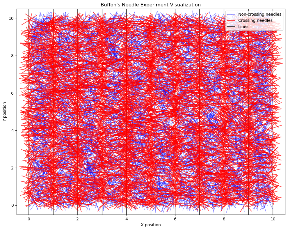
Visualization: We highlight crossing needles in red and non-crossing needles in blue.
Convergence Analysis: We track how our estimate approaches $\pi$ as we increase the number of needles, showing that Monte Carlo methods require large sample sizes for accuracy.

Full Code

import numpy as np
import matplotlib.pyplot as plt
from matplotlib.lines import Line2D
from tqdm import tqdm
from typing import Tuple, List, Optional, Dict, Any, Union, Callable

def simulate_buffon_needle(
    num_needles: int, 
    needle_length: float = 1, 
    line_distance: float = 1, 
    floor_width: float = 10
) -> Tuple[float, int, List[Tuple[float, float, float]]]:
    """
    Simulate Buffon's needle experiment.
    
    Parameters:
    -----------
    num_needles : int
        Number of needles to drop
    needle_length : float
        Length of each needle (should be <= line_distance)
    line_distance : float
        Distance between parallel lines
    floor_width : float
        Total width of the floor for visualization
    
    Returns:
    --------
    Tuple[float, int, List[Tuple[float, float, float]]]
        (estimated_pi, crossings, needles)
        where needles is a list of (x, y, theta) for each needle
    """
    # validate needle length
    if needle_length > line_distance:
        raise ValueError("Needle length must be less than or equal to line distance")
    
    # random positions and angles for needles
    # for visualization: x positions across the entire floor
    x_positions = np.random.uniform(0, floor_width, num_needles)
    thetas = np.random.uniform(0, np.pi, num_needles)
    
    # calculate y positions (0-10 for visualization)
    y_positions = np.random.uniform(0, 10, num_needles)
    
    # for calculation: find distance to nearest line for each needle
    # lines are at positions 0, line_distance, 2*line_distance, etc.
    nearest_line_positions = np.floor(x_positions / line_distance) * line_distance
    distances_to_nearest_line = x_positions - nearest_line_positions
    
    # determine which needles cross a line
    needle_half_length = needle_length / 2
    
    # a needle crosses a line if distance to nearest line < (L/2)*sin(theta)
    # or if distance to next line > line_distance - (L/2)*sin(theta)
    crossing_left = distances_to_nearest_line < needle_half_length * np.sin(thetas)
    crossing_right = distances_to_nearest_line > line_distance - needle_half_length * np.sin(thetas)
    crossings = np.sum(crossing_left | crossing_right)
    
    # calculate estimated π
    if crossings > 0:
        estimated_pi = (2 * needle_length * num_needles) / (crossings * line_distance)
    else:
        estimated_pi = float('inf')
    
    # prepare needle data for visualization
    needles = [(x_positions[i], y_positions[i], thetas[i]) for i in range(num_needles)]
    
    return estimated_pi, crossings, needles

def plot_experiment(
    needles: List[Tuple[float, float, float]], 
    line_distance: float = 1, 
    max_y: float = 10, 
    needle_length: float = 1, 
    highlight_crossings: bool = True
) -> plt.Figure:
    """
    Visualize the Buffon's needle experiment.
    
    Parameters:
    -----------
    needles : List[Tuple[float, float, float]]
        List of (x, y, theta) for each needle
    line_distance : float
        Distance between parallel lines
    max_y : float
        Maximum y value for visualization
    needle_length : float
        Length of each needle
    highlight_crossings : bool
        Whether to highlight needles that cross lines
        
    Returns:
    --------
    plt.Figure
        The matplotlib figure object
    """
    fig, ax = plt.subplots(figsize=(10, 8))
    
    # draw parallel lines
    num_lines = int(10 / line_distance) + 1
    for i in range(num_lines):
        ax.axvline(x=i*line_distance, color='black', linestyle='-', alpha=0.7)
    
    # half-length of the needle
    half_length = needle_length / 2
    
    # draw needles
    crossing_needles = []
    non_crossing_needles = []
    
    for x, y, theta in needles:
        # calculate needle endpoints
        dx = half_length * np.sin(theta)
        dy = half_length * np.cos(theta)
        
        x1, y1 = x - dx, y - dy
        x2, y2 = x + dx, y + dy
        
        # check if needle crosses a line
        crosses = False
        line_positions = [i*line_distance for i in range(num_lines)]
        for line_pos in line_positions:
            # if the needle endpoints are on opposite sides of the line
            if (x1 - line_pos) * (x2 - line_pos) <= 0:
                crosses = True
                break
        
        if crosses:
            crossing_needles.append([(x1, y1), (x2, y2)])
        else:
            non_crossing_needles.append([(x1, y1), (x2, y2)])
    
    # plot non-crossing needles
    for needle in non_crossing_needles:
        (x1, y1), (x2, y2) = needle
        ax.plot([x1, x2], [y1, y2], 'b-', alpha=0.5, linewidth=1)
    
    # plot crossing needles
    for needle in crossing_needles:
        (x1, y1), (x2, y2) = needle
        ax.plot([x1, x2], [y1, y2], 'r-', alpha=0.7, linewidth=1.5)
    
    # add legend
    legend_elements = [
        Line2D([0], [0], color='blue', lw=1.5, alpha=0.5, label='Non-crossing needles'),
        Line2D([0], [0], color='red', lw=1.5, alpha=0.7, label='Crossing needles'),
        Line2D([0], [0], color='black', lw=1.5, alpha=0.7, label='Lines')
    ]
    ax.legend(handles=legend_elements, loc='upper right')
    
    # set axis limits and labels
    ax.set_xlim(-0.5, (num_lines-1)*line_distance + 0.5)
    ax.set_ylim(-0.5, max_y + 0.5)
    ax.set_xlabel('X position')
    ax.set_ylabel('Y position')
    ax.set_title("Buffon's Needle Experiment Visualization")
    
    return fig

def run_buffon_experiment(
    max_needles: int = 10000, 
    step: int = 1000, 
    needle_length: float = 1, 
    line_distance: float = 1, 
    floor_width: float = 10
) -> Tuple[range, List[float]]:
    """
    Run Buffon's needle experiment with increasing numbers of needles.
    
    Parameters:
    -----------
    max_needles : int
        Maximum number of needles to simulate
    step : int
        Step size for increasing number of needles
    needle_length : float
        Length of each needle
    line_distance : float
        Distance between parallel lines
    floor_width : float
        Width of the entire floor for visualization
        
    Returns:
    --------
    Tuple[range, List[float]]
        (needle_counts, pi_estimates) where needle_counts is a range object
        and pi_estimates is a list of estimated π values
    """
    needle_counts = range(step, max_needles + step, step)
    pi_estimates = []
    errors = []
    
    for count in tqdm(needle_counts, desc="Simulating needle drops"):
        estimated_pi, _, _ = simulate_buffon_needle(count, needle_length, line_distance, floor_width)
        pi_estimates.append(estimated_pi)
        errors.append(abs(estimated_pi - np.pi)/np.pi * 100)  # calculate percentage error
    
    # plot results
    fig, ax1 = plt.subplots(1, 1, figsize=(12, 10), sharex=True)
    
    # plot 1: estimated π values
    ax1.plot(needle_counts, pi_estimates, 'b-', alpha=0.7)
    ax1.axhline(y=np.pi, color='r', linestyle='--', alpha=0.7, label=f'π = {np.pi:.6f}')
    ax1.set_ylabel('Estimated π')
    ax1.set_title('Estimated Value of π vs. Number of Needles')
    ax1.grid(True, alpha=0.3)
    ax1.legend()
    
    plt.tight_layout()
    
    return needle_counts, pi_estimates

# example usage
if __name__ == "__main__":
    np.random.seed(42)  # for reproducibility
    
    # simulation parameters
    needle_length = 0.8
    line_distance = 1.0
    floor_width = 10.0  # width of the entire floor
    
    # small visualization example
    num_needles_viz = 10000
    estimated_pi, crossings, needles = simulate_buffon_needle(
        num_needles_viz, 
        needle_length, 
        line_distance, 
        floor_width
    )
    print(f"Dropped {num_needles_viz} needles, {crossings} crossed lines")
    print(f"Estimated π = {estimated_pi:.6f} (Actual π = {np.pi:.6f})")
    
    # visualize the experiment
    fig = plot_experiment(needles, line_distance, 10, needle_length)
    plt.tight_layout()
    plt.savefig('buffon_needle_visualization.png', dpi=300)
    
    # run a larger experiment to see convergence
    needle_counts, pi_estimates = run_buffon_experiment(
        max_needles=100000, 
        step=1000, 
        needle_length=needle_length, 
        line_distance=line_distance
    )
    
    # print final estimate
    final_estimate = pi_estimates[-1]
    print(f"\nFinal estimate with {needle_counts[-1]} needles: π ≈ {final_estimate:.6f}")
    print(f"Error: {abs(final_estimate - np.pi):.6f} ({abs(final_estimate - np.pi)/np.pi*100:.4f}%)")
    
    plt.savefig('buffon_pi_convergence.png', dpi=300)
    plt.show()

Results and Convergence

When we run our simulation with an increasing number of toothpicks, we can observe something cool happening: our estimate of $\pi$ gradually converges to the true value as the sample size grows.

Here is the putput from running a simulation using 100000 toothpicks.

Desktop View

Here is the plot showing the numerical convergence to the value of $\pi$.

Desktop View

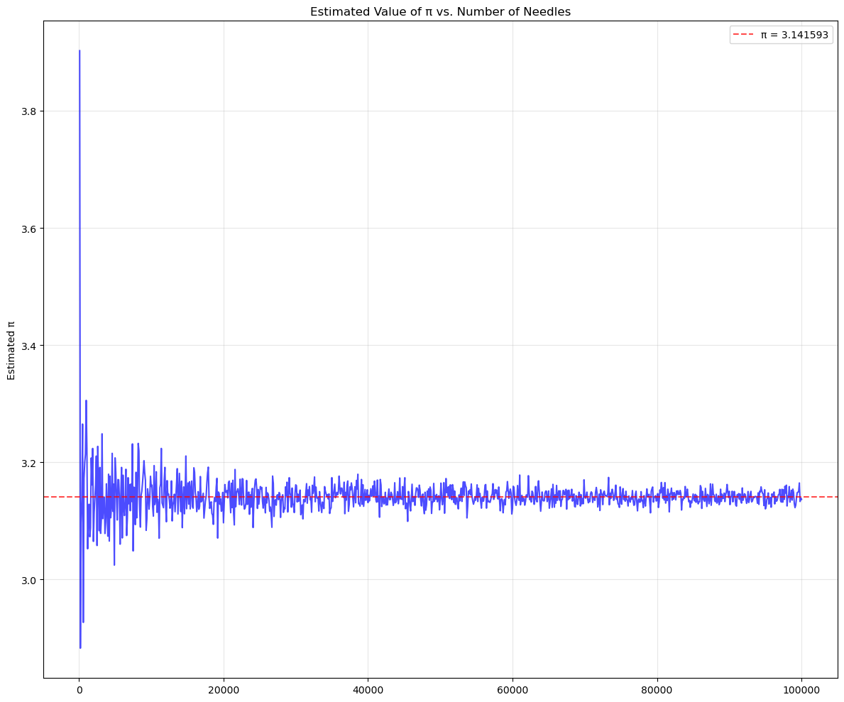
With just a few hundred toothpicks, our estimate might be off by 10% or more. But with tens of thousands of toothpicks, we typically get within 0.1% of the actual value of $\pi$.

Just for fun here is an animation showing the convergence of the value of $\pi$ as we drop more and more toothpicks.

Desktop View

Conclusion

I found this particular problem interesting owing to the overlap of probability and geometry. The fact that $\pi$, this transcendental number that appears throughout mathematics, can be approximated by simply dropping sticks on the floor is fascinating. I hope you enjoyed this breakdown of the problem and our implementation.

The next time you spill toothpicks on your kitchen floor, don’t just sweep them up. Count how many cross the tiles, and see how close you can approximate the value of $\pi$.

Deriving the Formula

Here we discuss how Buffon derived this equation. When Buffon solved this problem in the 18th century, he used geometric probability, a field that was relatively new at the time. His approach is very elegant hence I wanted to include it here.

Setting Up the Parameters:

The position of a toothpick can be completely described by two independent variables:
- The distance $x$ from the center of the toothpick to the nearest floorboard edge (ranges from 0 to $d/2$)
- The angle $\theta$ between the toothpick and the edge (ranges from 0 to $\pi$)

Geometric Analysis:

For any given angle $\theta$, the toothpick will cross between two floorboards if the distance from its centre to the nearest line is less than $\frac{l\sin\theta}{2}$
To visualize this: imagine a toothpick at angle $\theta$. The “reach” of this toothpick from its centre point is $(l/2)\sin\theta$ in the direction perpendicular to the lines.

Calculating the Probability:

For a fixed angle $\theta$, the toothpick crosses between two floorboards when
\[x < \frac{l\sin\theta}{2}\]
Since $x$ is uniformly distributed between 0 and $d/2$, the probability of crossing at this specific angle is
\[P(\text{crossing} | \theta) = \frac{l\sin\theta}{d}\]
To get the overall probability, we need to integrate this over all possible angles
\[P = \frac{2}{\pi} \int\limits_{0}^{\pi/2} \frac{l\sin\theta}{d} d\theta\]

The 2/$\pi$ factor comes from normalizing over the range of angles. Solving this integral

\[\begin{aligned} P &= \frac{2}{\pi} \frac{l}{d} \left[-\cos(\theta)\right]_{0}^{\pi/2} \\ P &= \frac{2}{\pi} \frac{l}{d} \left[0 - (-1)\right] \\ P &= \frac{2}{\pi} \frac{l}{d} 1 \\ P &= \frac{2l}{\pi d} \end{aligned}\]

What makes this result so elegant is that $\pi$ appears naturally in the calculation because:

The range of possible angles (0 to $\pi$) introduces a factor of $\pi$ in the denominator
The integration of $\sin\theta$ over this range brings in trigonometric properties related to circles
The averaging over all possible orientations essentially captures the ratio of a circle’s circumference to its diameter - which is precisely the definition of $\pi$

T>T: Buffon's Needle: Estimating π using Toothpicks

Try the code yourself!

The Problem

The Mathematics

Simulating the Experiment with Python

1. Imports and Setup

2. Needle Simulation Function

3. Animation Creation Function

4. Setting Up the Needle Plot

5. Setting Up the Convergence Plot

6. Initializing Plot Elements

7. Animation Initialization Function

8. Animation Update Function

9. Creating and Saving the Animation

10. Main Code Execution

Key Concepts in the Implementation

Full Code

Results and Convergence

Conclusion

Deriving the Formula

Recent Update

Trending Tags

Contents

Trending Tags

T>T: Buffon's Needle: Estimating π using Toothpicks

Try the code yourself!

The Problem

The Mathematics

Simulating the Experiment with Python

1. Imports and Setup

2. Needle Simulation Function

3. Animation Creation Function

4. Setting Up the Needle Plot

5. Setting Up the Convergence Plot

6. Initializing Plot Elements

7. Animation Initialization Function

8. Animation Update Function

9. Creating and Saving the Animation

10. Main Code Execution

Key Concepts in the Implementation

Full Code

Results and Convergence

Conclusion

Deriving the Formula

Recent Update

Trending Tags

Contents

Further Reading

T>T: Langton's Ant 2: Electric Boogaloo

T>T: Brownian Motion

T>T: Writing and Running Python Programs Locally

Trending Tags