T>T: Exact Cusp–Tail Density Functional for the Bound Two-Electron Coulomb Series
My background is in physics and when I entered the weird and wonderful world of chemistry, I remember reading about the Hohenberg and Kohn theorem which has been floating around my head ever since. If you ever see me sitting quietly in a corner, I am probably thinking about this problem, or just staring at the wall but hopefully the former. The TLDR of this theorem is:
“the ground-state properties of a many-electron system are uniquely determined by its electron density rather than its complex quantum wave function.”
This blew my mind as the proof is trivial yet its consequences, in my opinion, are not. I have been captivated by this and have been thinking of ways of finding this elusive relationship between the electron density and the exact energy of a fully correlated two-electron atom which taps into my background in this subfield. My original instinct was to look in the middle of the density: its moments, its maximum, its shape, and combinations of these discovered by symbolic regression. That remains an interesting problem, but it led me to ask a slightly perverse question:
What if the middle of the density is unnecessary?
Recently I have found myself thinking back to how black holes store information with their entropy changing with their surface area and not their volume. This leads me to try and pose a problem in terms of some form of dimensionality reduction or looking at extrema points rather than the entire space and seeing if the important information is contained there.
At the nucleus the density has a cusp. Infinitely far from the nucleus it has an exponentially small tail. These look like two unrelated pieces of boundary information, but together they contain exactly the two numbers needed to reconstruct the total energy. The cusp reveals the nuclear charge $Z$; the tail reveals the first ionisation energy $I$; and the ion left after removing one electron is hydrogenic, with the exactly known energy $-Z^2/2$.
The result is
\[\boxed{ E_2[\rho] = -\frac{1}{2} \left[-\frac{\rho'(0)}{2\rho(0)}\right]^2 -\frac{1}{8} \left[ \lim_{r\rightarrow\infty}\frac{\log\rho(r)}{r} \right]^2 }.\]in atomic units. It is exact for the bound ground-state densities of the helium-like Coulomb series.
There is a catch, and it is important. This is not the universal Levy-Lieb functional, and the tail is not a magical shortcut around solving the quantum problem: the ionisation energy is encoded in an exponentially small part of the density that is numerically difficult to obtain. For me at least the formula is simultaneously exact, simple and rather awkward. That combination is precisely why I find it interesting. That and I have not seen this form presented anywhere before; if you have feel free to send me a message.
The system and the claim
Consider a point nucleus of charge $Z$, two electrons, an infinitely heavy nucleus, and the non-relativistic Hamiltonian
\[\hat H_Z = -\frac{1}{2}\nabla_1^2 -\frac{1}{2}\nabla_2^2 -\frac{Z}{r_1} -\frac{Z}{r_2} +\frac{1}{r_{12}}.\]Let $E_2(Z)$ be its ground-state energy and let $\rho_Z(r)$ be the spherically averaged, spin-summed one-electron density, normalised as
\[4\pi\int_0^\infty r^2\rho_Z(r)\,dr=2.\]The domain matters. I am considering only densities actually generated by normalisable ground states of this Hamiltonian:
\[\mathcal D_{2,\mathrm{Coul}}^{\mathrm{gs}} = \left\{ \rho_Z:\rho_Z\text{ is the bound ground-state density of }\hat H_Z, \ Z>Z_c \right\},\]where $Z_c\approx0.9110282241$ is the critical charge for binding the second electron. The proposed map is therefore
\[E_2:\mathcal D_{2,\mathrm{Coul}}^{\mathrm{gs}}\longrightarrow\mathbb R.\]This restricted domain is not fine print added after this derivation. It is what makes the statement true. An arbitrary positive function normalised to two electrons can have any origin slope and any tail slope; those two numbers need not belong to a common Coulomb Hamiltonian. On the physical manifold they are compatible because the same Hamiltonian produced both.
Boundary one: the cusp tells us $Z$
A Coulomb potential is singular at the nucleus. The kinetic energy must cancel that singularity, forcing the exact wavefunction to develop the electron–nucleus cusp described by Kato.
For the spherically averaged density the corresponding cusp theorem is
\[\rho_Z'(0)=-2Z\rho_Z(0).\]Therefore
\[\boxed{ Z[\rho]= -\frac{\rho'(0)}{2\rho(0)} }.\]The density normalisation cancels, which is useful. The spherical averaging is important: Kato’s original wavefunction condition is itself an angular-average statement. I originally wrote it as a pointwise radial identity and differentiated under the integral, which is a useful formal mnemonic but is not the cleanest proof. The density cusp theorem is the rigorous statement we need.
There is also an easy numerical trap here. Most atomic calculations store the radial distribution
\[D(r)=4\pi r^2\rho(r),\]not $\rho(r)$ itself. Since $D(0)=0$, the ratio $D’(0)/D(0)$ is meaningless. We must first remove the geometrical $4\pi r^2$, or use an equivalent small-$r$ expansion.
Near the origin,
\[\rho(r)=\rho(0)\left(1-2Zr+O(r^2)\right),\]and hence
\[\frac{D(r)}{r^2} =4\pi\rho(0)-8\pi Z\rho(0)r+O(r^2).\]If a polynomial fit gives
\[\frac{D(r)}{r^2}=c_0+c_1r+c_2r^2+\cdots,\]then the charge follows without numerically differentiating noisy density values:
\[Z=-\frac{c_1}{2c_0}.\]This is the form I use in the numerical experiment below.
Boundary two: the tail tells us $I$
The first ionisation energy is
\[I(Z)=E_1(Z)-E_2(Z),\]where $E_1$ is the energy of the one-electron daughter ion. Exact asymptotic results for many-electron densities connect this spectral gap to the exponential decay of the density; see the work of Hoffmann-Ostenhof, Hoffmann-Ostenhof and Ahlrichs and Almbladh and von Barth.
The conservative statement is
\[\lim_{r\rightarrow\infty}\frac{1}{r}\log\rho_Z(r) =-2\sqrt{2I(Z)}.\]Define the positive density decay constant
\[\kappa=2\sqrt{2I}.\]Then
\[\boxed{I[\rho]=\frac{\kappa[\rho]^2}{8}}.\]Why the factor of two? The outer-electron amplitude falls approximately as
\[e^{-\sqrt{2I}\,r},\]whereas the density is quadratic in that amplitude and therefore falls as
\[e^{-2\sqrt{2I}\,r}.\]For the refined Coulomb tail
\[\rho(r)=A r^\beta e^{-\kappa r}\left(1+o(1)\right),\]we expect
\[\frac{d}{dr}\log\rho(r)=\frac{\beta}{r}-\kappa+o(1),\]and hence
\[\kappa[\rho] =-\lim_{r\rightarrow\infty}\frac{d}{dr}\log\rho(r).\]There is a small but real mathematical subtlety here. We cannot differentiate an unspecified $o(1)$ remainder and automatically obtain another $o(1)$ remainder. The logarithmic-derivative formula therefore requires a derivative-controlled refined asymptotic expansion, or an independent theorem establishing that derivative limit (answers on a postcard from the mathematicians please). The exponential-rate form involving $r^{-1}\log\rho$ is, in my opinion at least, the safer theorem and is sufficient to establish the energy identity. I will use the derivative form when discussing smooth Coulomb tails, but the rate form is the logical foundation.
The daughter ion completes the argument
Removing one electron leaves a hydrogenic ion:
\[\hat H_1(Z)=-\frac{1}{2}\nabla^2-\frac{Z}{r}.\]Its ground-state energy is exactly
\[E_1(Z)=-\frac{Z^2}{2}.\]Since $I=E_1-E_2$,
\[E_2=E_1-I=-\frac{Z^2}{2}-I.\]Substituting the two density invariants gives
\[E_2[\rho] = -\frac{1}{2} \left[-\frac{\rho'(0)}{2\rho(0)}\right]^2 -\frac{1}{8} \left[ \lim_{r\rightarrow\infty}\frac{d}{dr}\log\rho(r) \right]^2.\]Or, using only the conservative exponential-rate theorem,
\[\boxed{ E_2[\rho] = -\frac{1}{2} \left[-\frac{\rho'(0)}{2\rho(0)}\right]^2 -\frac{1}{8} \left[ \lim_{r\rightarrow\infty}\frac{\log\rho(r)}{r} \right]^2 }.\]The signs are worth checking. Both terms must be negative. For helium, $Z=2$ gives the hydrogenic threshold $-2\,E_h$, and $I\approx0.9037\,E_h$, so
\[E_2\approx-2-0.9037=-2.9037\,E_h,\]as expected.
Is this a genuine density functional, or a tautology?
My verdict on this is: it is a genuine restricted density functional, and it is also close to a spectral identity written in the language of density.
The cusp alone already identifies $Z$, so on this one-parameter family it identifies the external potential. The Hohenberg-Kohn theorem then tells us that the ground-state density determines the energy. The new formula makes that map explicit, but the tail contains $I$, and $I=E_1-E_2$ already contains the unknown energy. We have not made the many-electron problem computationally disappear; we have found precisely where the answer is stored in the density.
That is why I do not claim this the exact universal density functional. The universal Levy-Lieb object is
\[F[\rho]=\min_{\Psi\rightarrow\rho} \langle\Psi|\hat T+\hat V_{ee}|\Psi\rangle,\]defined on a much larger set of densities and independent of the external potential. The cusp-tail expression instead gives the total energy on a particular physical manifold. It does not separately provide $T_s[\rho]$, $V_{ee}[\rho]$, $E_c[\rho]$, or a useful approximation for arbitrary trial densities.
One can construct the corresponding restricted internal energy on this same manifold. Since
\[V_{ne}[\rho]=-Z[\rho]\int\frac{\rho(\mathbf r)}{r}\,d\mathbf r,\]we have
\[F_{\mathrm{Coul}}[\rho] =E_2[\rho] +Z[\rho]\int\frac{\rho(\mathbf r)}{r}\,d\mathbf r.\]This is exact on $\mathcal D_{2,\mathrm{Coul}}^{\mathrm{gs}}$, but it is still not an extension of the universal Levy-Lieb functional to arbitrary densities.
Can we remove the limit?
The limit at infinity is analytical but unpleasant. A finite grid never reaches infinity, and by the time the true asymptotic regime is reached the density may be many orders of magnitude below its maximum.
There is no exact replacement using the density and a finite number of derivatives at one finite radius. Two functions can agree perfectly on every finite interval we inspect and still have different asymptotic exponents beyond it. Removing all dependence on the far tail would remove the information that determines $I$.
We can, however, write an exactly equivalent expression with no explicit limit. Define the exponential moment generating integral
\[M_\rho(s)=\int_{\mathbb R^3}e^{s|\mathbf r|}\rho(\mathbf r)\,d\mathbf r =4\pi\int_0^\infty r^2e^{sr}\rho(r)\,dr,\]and define its abscissa of convergence
\[\kappa_\star[\rho] = \sup\left\{ s\geq0:M_\rho(s)<\infty \right\}.\]If $\rho(r)\sim Ar^\beta e^{-\kappa r}$, then $M_\rho(s)$ converges for $s<\kappa$ and diverges for $s>\kappa$. Whether it converges at the single boundary point $s=\kappa$ does not change the supremum. Therefore
\[\kappa_\star[\rho]=\kappa[\rho]=2\sqrt{2I},\]and the energy may be written as
\[\boxed{ E_2[\rho] = -\frac{1}{2} \left[-\frac{\rho'(0)}{2\rho(0)}\right]^2 -\frac{1}{8}\kappa_\star[\rho]^2 }.\]This is a limit-free analytical form. It replaces a pointwise asymptotic slope with the convergence boundary of an integral transform. I prefer this form because it says something precise: the ionisation energy is the radius of exponential integrability of the density.
It does not make the numerical problem vanish (annoyingly). Locating a convergence boundary from truncated data is still an asymptotic inference and is arguably less convenient than fitting the tail directly. The infinity has moved from a displayed limit into the domain of an integral; it has not been abolished.
A numerical test from independently calculated densities
A numerical experiment cannot prove an exact identity. What it can do is test whether two boundary quantities extracted from tabulated density data reconstruct reference variational eigenvalues that were not used in the extraction.
I used fully correlated radial densities for nine members of the two-electron Coulomb series,
\[Z\in\{0.95,1.0,1.1,1.5,2,3,5,8,10\}.\]For each density I performed three steps.
- I fitted $D(r)/r^2$ close to the origin and obtained $Z=-c_1/(2c_0)$. This avoids pointwise numerical differentiation.
I fitted the large-$r$ radial distribution to the Coulomb asymptotic form. If $q=\sqrt{2I}$ and $\kappa=2q$, the outer electron sees the residual charge $Z-1$, giving
\[D(r)\sim C r^{4(Z-1)/\kappa}e^{-\kappa r} \left(1+\frac{a_1}{r}+\cdots\right).\]I fitted $\log D(r)$ in several density windows, included one $1/r$ correction, and selected a stable adjacent-window plateau. The selection used the density alone; the reference energy never entered the fit.
I then evaluated
\[E_{\mathrm{density}}=-\frac{Z_{\mathrm{cusp}}^2}{2}-\frac{\kappa_{\mathrm{tail}}^2}{8}\]and only then compared it with the fully correlated variational eigenvalue from the underlying wavefunction calculation.
The full calculation is already implemented in previous work I have done in what I called density-energy space, so I reused that path rather than writing a second validation script. Re-running it gives a median charge error of $9.36\times10^{-6}$, a median tail-exponent error of $1.20\times10^{-4}$, a median energy error of $1.05\times10^{-4}\,E_h$, and a worst energy error of $3.75\times10^{-4}\,E_h$.
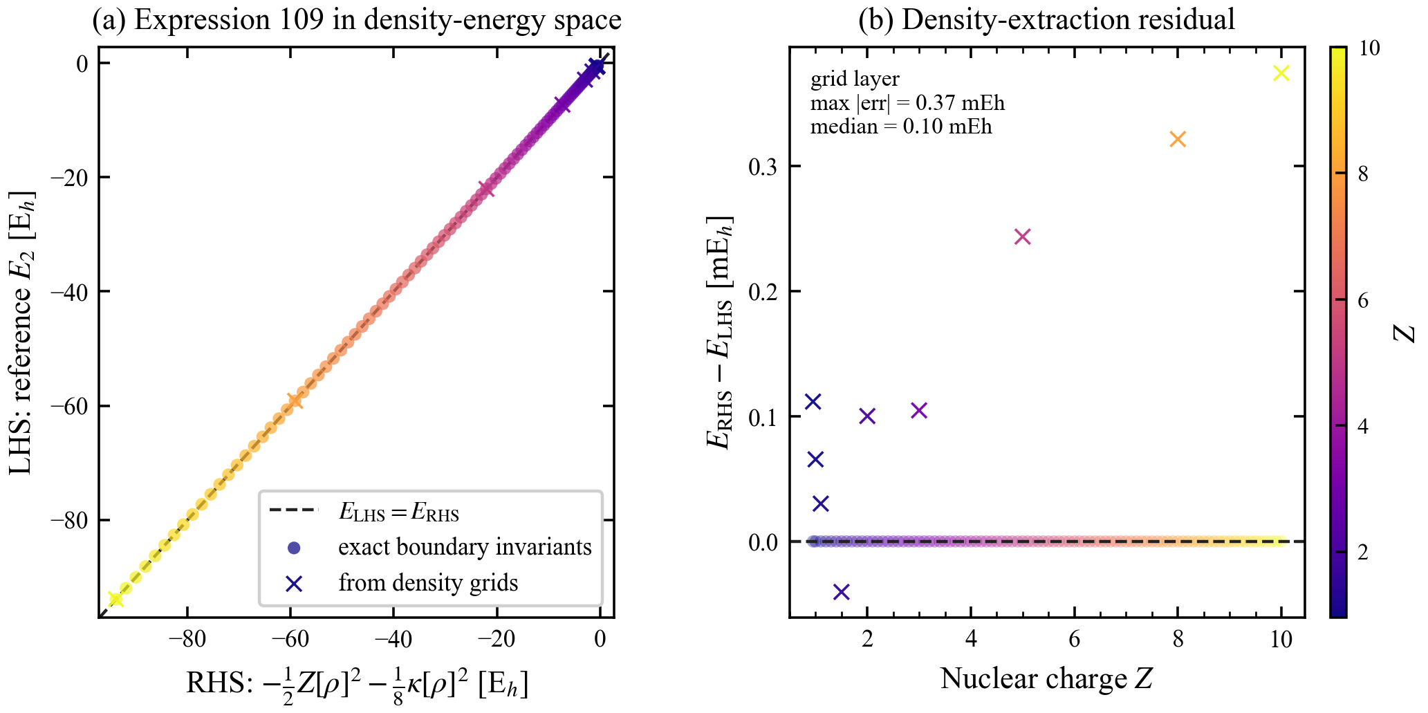
The left panel is visually boring: the reconstructed and reference energies lie on the diagonal over nearly two orders of magnitude. The residual panel is more informative where it shows the small but nonzero error caused by extracting boundary invariants from finite density grids.
The pale circular layer uses the exact boundary invariants implied by the reference energies, so it checks only the algebra. The nine crosses are the meaningful numerical test: their cusp and tail values come from the density grids with no reference energy supplied to either fit.
Some representative values are:
| $Z$ | $Z$ from cusp | $\kappa$ from tail | $E_{\mathrm{density}}/E_h$ | $E_{\mathrm{reference}}/E_h$ | error / m$E_h$ |
|---|---|---|---|---|---|
| 0.95 | 0.94993084 | 0.29432790 | -0.46201291 | -0.46212470 | +0.1118 |
| 1.00 | 0.99991417 | 0.47134892 | -0.52768540 | -0.52775102 | +0.0656 |
| 1.50 | 1.49999398 | 1.65003882 | -1.46531948 | -1.46527905 | -0.0404 |
| 2.00 | 1.99999520 | 2.68869294 | -2.90362412 | -2.90372438 | +0.1003 |
| 3.00 | 2.99999264 | 4.71578687 | -7.27980866 | -7.27991341 | +0.1048 |
| 5.00 | 4.99999223 | 8.73190321 | -22.03072786 | -22.03097158 | +0.2437 |
| 8.00 | 7.99999064 | 14.73942964 | -59.15627339 | -59.15659512 | +0.3217 |
| 10.00 | 9.99996205 | 18.74178464 | -93.90643194 | -93.90680651 | +0.3746 |
The remaining error is not evidence against the identity. The cusp is recovered very accurately; the tail dominates the uncertainty. That is exactly what we should expect. A variational wavefunction can give an excellent total energy while still representing an exponentially tiny tail imperfectly, and a finite radial box forces us to decide where the asymptotic regime begins.
What I think the result means
I began this investigation hoping that the energy might be encoded in a compact set of ordinary density moments. Instead, the cleanest exact answer I have found thus far lives at the two most inconvenient places possible; one point at the nucleus and the other the limit of vanishing density infinitely far away.
That is not the universal functional sought in practical DFT, and it is not an efficient black-box energy algorithm. But I do think it is more than an empty rewriting. It gives a constructive picture of how the density identifies both the external Coulomb field and the spectral position of the many-electron ground state:
\[\rho \longrightarrow \left( Z\text{ from the cusp}, I\text{ from the tail} \right) \longrightarrow E_2=-\frac{Z^2}{2}-I.\]The density’s shortest-distance behaviour tells us which Hamiltonian we have. Its longest-distance behaviour tells us how far the ground state lies below ionisation. The entire total energy is the bridge between those two boundaries.
So, is it trivial or interesting? My current answer is both. Once written down, the algebra is almost embarrassingly short. Recognising that the two ends of the exact density supply exactly the two required spectral invariants is the interesting part. And the numerical experiment shows that it holds for a range of nuclear charges. For the single reader this post will get, what do you think?