T>T: Helium to 60 Significant Figures with FLAKE, The Full Story

Posted Aug 25, 2026

The ceiling reached by each approach on the way to 60 significant figures.

By Adam Baskerville

views 77 min read

T>T: Helium to 60 Significant Figures with FLAKE, The Full Story

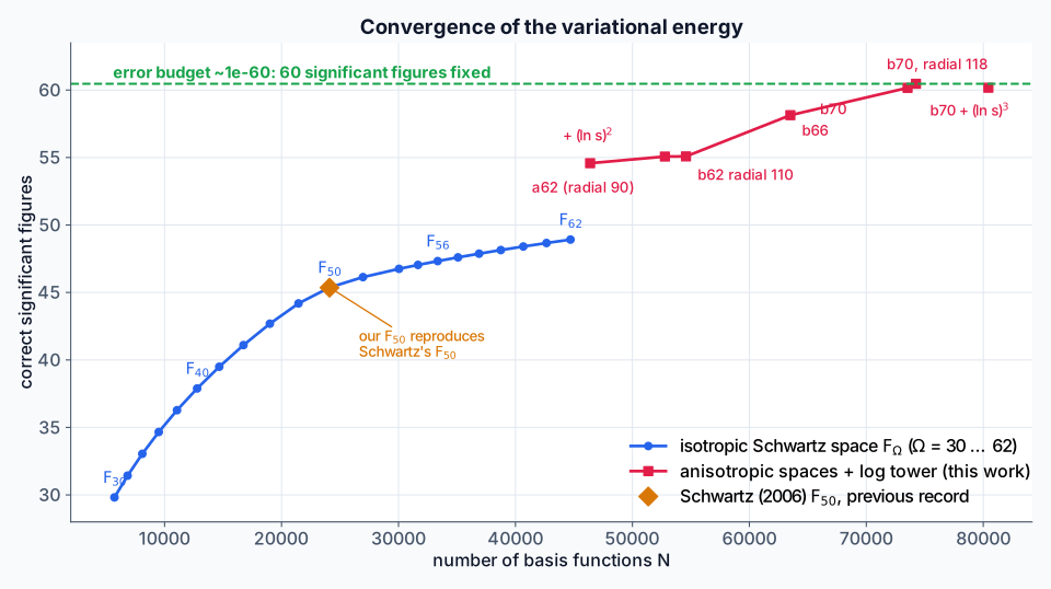
TLDR: In this post learn how to calculate a rigorous variational upper bound on the non-relativistic ground-state energy of helium, correct to 60 significant figures, computable on your laptop! This surpasses the previous record value (Schwartz, 2006) correct to 44 which stood for 20 years.

The result (in hartrees)

Schwartz (2006), previous record

−2.903724377034119598311159245194404446696925309838

This work (2026), certified

−2.903724377034119598311159245194404446696925311117290339042346702…

Introduction

This ended up being one of the longest posts I have ever written; but I also figured out that there is a way to add an image to the post link on the main page, snazzy!

Will I publish this result? No, because who cares and I do not want to pay the journal fees for a paper only five people might read. All the code needed to replicate this work is available on GitHub.

The obvious first question you may have from the TLDR is, “why do we need to know the non-relativistic, time independent helium energy to such high accuracy?” and the answer is that we do not. In fact the number is physically incorrect as past ~10 digits relativistic effects and quantum electrodynamic effects, QED, become significant which alters the value.

The aim of this post is to explain and hopefully convince you that it was infact a good use of my spare time (significantly more spare time than I had planned…) and that there is a lot to learn from such an exercise.

At Kvantify we work on solving the most challenging problems in chemistry and biology with speed and precision in order to discover molecules that cure diseases. This is no simple task and often involves dramatically improving the computational speed or accuracy of the algorithms which we develop. Setting oneself a challenge such as the topic in this post, forces us to think outside of the box, to innovate and to learn; learnings which will translate into new ideas and applications that we work on.

I have worked in the field of high accuracy quantum chemical calculations for many years but in order to solve this problem, I had to learn new techniques and ideas which I highlight as we go through. You might not work in the field of quantum mechanics, so I want you to be able to take away some useful ideas or techniques which you might apply to your own work.

Why not use AI?

Artificial intelligence, AI, is very much the buzzword of the last 5 years and it is prudent to ask why not just ask AI to solve it for us.

I seldom use AI in my personal projects as they are just fun problems I work on in my spare time as a means of bettering my own understanding of a certain topic. I am very transparent when I do use it and there is no AI used in the solution to this problem, however I did test Codex and Claude to see if they could find a way of solving it.

Interestingly they both failed and exhibited similar behaviours. They would formulate a sensible plan of attack and then implement and test it. When it did not achive the desired accuracy they would both get stuck trying to iterate and improve the initial idea they chose. Neither of them would re-evaluate their plan based on what the results were showing when you could see that there was no conceivable way to achieve the required precision. They did both however successfully implement methods which achieved very good accuracy (> 20 digits).

I am no prompt engineer so maybe someone else can design a better prompt to guide them but as I am also under a hosepipe ban here in Cambridgeshire due to the droughts we experienced over summer, I feel this extends to running AI tools hosted in some datacentre, wasting untold amounts of water.

Birds-eye view

I love a good deep dive so this post is aimed to be one. If you still have questions then feel to message me.

A rough guide to this post is as follows

Part I sets up the problem,
Part II is the method in full detail,
Part III is the road that led there
Part IV is the result and its error analysis,
Part V is the code and the optimisations that made it fast,
Part VI collects the lessons, including what I think transfers to other fields

If you only want to read about the development and implementation of the working method, you only need read Parts I and II.

Part III documents the numerous pathways and deadends that I explored on the way to the solution. Scienctific progress is rarely one-shoted in an afternoon from a single hypothesis and I feel it is disingenuous that we often pretend it is.

The latter parts are concerned with error analysis, the code and a summary of what I learned along the way.

Why anyone computes this

Helium has played a significant role in the field of quantum chemistry over the last century as it represents the simplest, most complex many body problem that contains electron correlation. The hydrogen atom, a two-particle system, is exactly solvable, but we do not yet possess the knowledge to solve the many-body Schrodinger equation exactly hence the field of quantum chemistry is built on numerical approximations to the time independent Schrodinger equation (TISE).

Hydrogen separates. Helium does not, because the electron–electron repulsion $1/r_{12}$ couples everything. In atomic units, with the nucleus fixed

\[H \;=\; -\tfrac12\nabla_1^2 \;-\; \tfrac12\nabla_2^2 \;-\; \frac{2}{r_1} \;-\; \frac{2}{r_2} \;+\; \frac{1}{r_{12}} .\]

So why do we still study this humble atom?

The origins of the LYP functional, one of the most popular correlation functionals used in approximate density functional theory (DFT), are firmly rooted in the helium atom based on previous work from Colle and Salvetti. This functional is used in over 40 different exchange–correlation functionals, including the ubiquitous B3LYP functional
The helium atom is “exactly solved” numerically which means we can gain insight into electron correlation, electron densities, Coulomb holes and more which acts as a foundation for when we move to larger atoms and molecules
The answer is unique, the Hamiltonian is exact, and everyone computes the same number. If your method, basis or linear algebra is subtly wrong, helium will tell you. Almost every technique for explicitly correlated few-body calculations was first proved on helium
From past experience, it is a model problem for singular eigenproblems. The wavefunction has cusps and logarithmic singularities. That makes the problem a clean test of how to approximate non-smooth solutions to high levels of precision. I have learned a lot of numerical techniques and methods from having to solve these kinds of differential equations as they will fight you every step of the way

A century of chasing digits

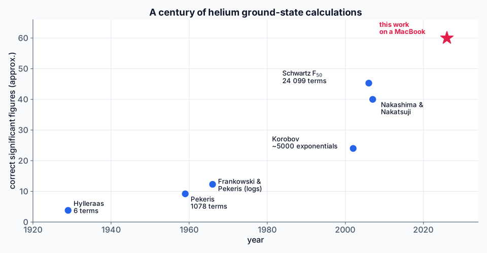Approximate correct significant figures over time. Each jump came from representing a missing piece of the exact wavefunction.

Year	Who	Key idea	Accuracy
1929	Hylleraas	put $r_{12}$ in the wavefunction	~4 significant figures with 6 terms
1954	Fock	triple-coalescence logarithms	explains slow convergence
1959	Pekeris	perimetric coordinates, recursion, 1078 terms on WEIZAC	~10 significant figures
1966	Frankowski & Pekeris	add $\ln s$ terms to the basis	~13 significant figures
2002	Korobov	thousands of quasi-random exponentials	~24 significant figures
2006	Schwartz	the $F_\Omega$ basis: negative powers and $\ln s$, $F_{50}$ with 24,099 terms	44 significant figures (error $1.3\times10^{-45}$)
2007	Nakashima & Nakatsuji	free iterative complement interaction	40+ significant figures
2026	this work	Kronecker white chart, anisotropic log tower	60 significant figures, certified

Schwartz’s 2006 calculation stood for twenty years. His $F_{50}$ value is correct to about $1.3\times10^{-45}$: our certified bound lies that below it.

Initial Thought Process

When I read content similar to this post you are reading now, I like to gain insight into the author’s thought process. The solution is interesting, but the way people approach and solve problems often influences the way I think about problems more generally. When I first started tackling this problem, I wrote down a list of bullet points summarising my thought process and proposed method of solution in my notebook which I include below. I also comment on whether my thought process ended up being correct or not.

Goal: Helium WR energy on a laptop with new, small basis set
Need: Basis, eigensolver, custom datatypes
Macbook memory will not store full matrices in TISE, need matrix free method (Correct!)
Use OctDouble precision, OD, as unevaluated sum of 8, 64-bit IEEE numbers (Incorrect. This surprised me the most as I routinely use this principle for high precision calculations as it is much faster than arbitrary precision data types but I found a much better way of doing it)
Definitely need logarithms in basis (Correct!)
LOBPCG method for solving? (Incorrect)
Generalised Schur decomposition maybe? (Incorrect)
Need preconditioner as everything will be linearly dependent and rubbish (Correct!)
Do not get tricked by basis sets that show great convergence early on, it is the plateau we need to look out for (Correct, this was one of the most frustrating hurdles in the entire project)
Probably hyper optimised C++ code to tackle the computational speed problem (Incorrect! This was also surprising. I did write a lot of custom eigen3 C++ code with custom datatypes, but the final version did not actually need it. I will however add this into a repository somewhere)

Part I: The problem

1. The Hamiltonian

For helium with the nucleus clamped at the origin (infinite nuclear mass), no relativity and no QED, the Hamiltonian in atomic units (hartree, bohr) is

\[H \;=\; -\tfrac12\nabla_1^2 \;-\; \tfrac12\nabla_2^2 \;-\; \frac{Z}{r_1} \;-\; \frac{Z}{r_2} \;+\; \frac{1}{r_{12}}, \qquad Z = 2 .\]

Here $r_i = \vert\mathbf r_i\vert$ and $r_{12} = \vert\mathbf r_1-\mathbf r_2\vert$. We want the lowest eigenvalue $E_0$ of the spatially symmetric (singlet) sector.

This model is not “real helium”. Real helium needs recoil (finite nuclear mass), relativistic, QED and nuclear-size corrections, each computed as an expectation value or perturbation built on top of the non-relativistic solution. For comparison with experiment, perhaps 10 digits of the non-relativistic energy are needed.

Everything beyond that is about the method and the computation; can we control a singular three-body eigenproblem to arbitrary precision, and what does it take? That makes helium the standard benchmark of explicitly correlated methods, and a model problem for singular PDE eigenvalue computation in general.

2. The benefit of the variational principle

For any normalisable trial function $\Psi$ in the domain of $H$,

\[E[\Psi] \;=\; \frac{\langle\Psi\vert H\vert\Psi\rangle}{\langle\Psi\vert\Psi\rangle} \;\ge\; E_0 .\]

Expand $\Psi = \sum_{\mu=1}^N c_\mu \phi_\mu$ in a basis and minimise over $c$. You get the generalised symmetric eigenproblem

\[\mathbf H\,c = E\,\mathbf S\,c, \qquad \mathbf H_{\mu\nu} = \langle\phi_\mu\vert H\vert\phi_\nu\rangle, \qquad \mathbf S_{\mu\nu} = \langle\phi_\mu\vert\phi_\nu\rangle .\]

Two classical facts carry the whole calculation:

Upper bound. The lowest eigenvalue $E^{(N)}$ is an upper bound on $E_0$. More generally (Hylleraas–Undheim–MacDonald), the $k$-th Ritz value bounds the $k$-th exact eigenvalue from above.
Monotonicity. If $V_N \subset V_{N'}$ then $E^{(N')} \le E^{(N)}$. Adding functions can never make things worse. This is why a sequence of nested spaces gives a clean convergence series.

This is the core idea behind everything here. If I hand you an explicit function and you can evaluate its Rayleigh quotient exactly, you have a rigorous upper bound, whatever solver produced the function. Expand $\Psi$ in $N$ basis functions and minimise. You get the generalised eigenproblem $Hc = ESc$, and adding functions can only lower the bound without going below the true value. We love variational problems for this reason, unfortunately it is often very difficult to pose a problem to be truly variational.

3. Reducing to three variables

The ground state has total angular momentum $L=0$ and an $S$-state wavefunction depends only on the three inter-particle distances $r_1, r_2, r_{12}$; the remaining three coordinates (the orientation of the triangle formed by the nucleus and the two electrons) integrate out. The six-dimensional volume element reduces to

\[d^3\mathbf r_1\, d^3\mathbf r_2 \;\longrightarrow\; 8\pi^2\, r_1 r_2 r_{12}\; dr_1\, dr_2\, dr_{12},\]

over the region allowed by the triangle inequality, $\vert r_1 - r_2\vert \le r_{12} \le r_1 + r_2$.

Now change to Hylleraas coordinates

\[s = r_1 + r_2, \qquad t = r_1 - r_2, \qquad u = r_{12}.\]

Then $r_1 = (s+t)/2$, $r_2 = (s-t)/2$, $r_1 r_2 = (s^2-t^2)/4$, and $dr_1\,dr_2 = \tfrac12\,ds\,dt$. The volume element becomes

\[d\tau \;=\; \pi^2\, u\,(s^2 - t^2)\; ds\, dt\, du, \qquad 0 \le \vert t\vert \le u \le s < \infty .\]

The constant $\pi^2$ cancels in every Rayleigh quotient, so from now on the weight is simply $W = u(s^2-t^2)$. Exchanging the electrons maps $t\to -t$, so the singlet ground state is even in $t$.

4. The energy functional in gradient form

We represent the kinetic energy using the symmetric first-derivative form,

\[\langle\Psi\vert T\vert\Psi\rangle = \tfrac12\int\big(\vert\nabla_1\Psi\vert^2 + \vert\nabla_2\Psi\vert^2\big)\,d\tau .\]

This is important, the “Laplacian” form $\langle\Psi\vert -\tfrac12\nabla^2\Psi\rangle$ is equal to it only when boundary terms vanish, and for functions containing $\ln s$ they need not vanish at the origin.

Unfortunately I learned this the hard way, but you don’t have to (Part III, Chapter 2 for more info): a second-derivative kinetic operator that was perfectly correct for polynomials gave wrong energies for log-singular functions. The following gradient form is boundary-safe.

For $\Psi(r_1,r_2,r_{12})$ the chain rule gives

\[\nabla_1\Psi = \Psi_{r_1}\hat{\mathbf r}_1 + \Psi_{r_{12}}\hat{\mathbf r}_{12}, \qquad \nabla_2\Psi = \Psi_{r_2}\hat{\mathbf r}_2 - \Psi_{r_{12}}\hat{\mathbf r}_{12},\]

with $\hat{\mathbf r}_{12} = (\mathbf r_1-\mathbf r_2)/r_{12}$. The dot products follow from the law of cosines, for example $\hat{\mathbf r}_1\cdot\hat{\mathbf r}_{12} = (r_1^2 + r_{12}^2 - r_2^2)/(2r_1r_{12})$. Substitute $\Psi_{r_1} = \Psi_s + \Psi_t$, $\Psi_{r_2} = \Psi_s - \Psi_t$ and $\Psi_{r_{12}} = \Psi_u$, multiply by the weight, and simplify. The result is:

\[E[\Psi] = \frac{\mathcal N[\Psi]}{\mathcal D[\Psi]}, \qquad \mathcal D[\Psi] = \int u(s^2-t^2)\,\Psi^2\,ds\,dt\,du,\] \[\begin{aligned} \mathcal N[\Psi] = \int \Big[\, & u(s^2-t^2)\big(\Psi_s^2+\Psi_t^2+\Psi_u^2\big) + 2s(u^2-t^2)\,\Psi_s\Psi_u \\ & + 2t(s^2-u^2)\,\Psi_t\Psi_u + \big(s^2-t^2-4Zsu\big)\,\Psi^2 \,\Big]\,ds\,dt\,du . \end{aligned}\]

The potential term also deserves mention, since $\frac1{r_1}+\frac1{r_2} = \frac{r_1+r_2}{r_1r_2} = \frac{4s}{s^2-t^2}$, multiplying the potential by the weight gives

\[u(s^2-t^2)\left[-Z\left(\frac1{r_1}+\frac1{r_2}\right) + \frac1u\right] = -4Zsu + s^2 - t^2 ,\]

which is a polynomial. The same is true of all the kinetic weights, every singular $1/r$ has been absorbed by the measure, which is what makes exact integration possible.

Quick sanity check to do by hand. Take $\Psi = e^{-\alpha s}$, a product of two hydrogen-like orbitals. Then $\Psi_s=-\alpha\Psi$ and $\Psi_t=\Psi_u=0$, and the functional gives $E(\alpha) = \alpha^2 - 2Z\alpha + \tfrac58\alpha = \alpha^2 - \tfrac{27}{8}\alpha$. The minimum is at $\alpha = 27/16$ with $E = -729/256 = -2.84765625$, the textbook screened-hydrogen result. Every code in this project was first checked against exactly this number.

5. Why helium is hard: cusps and logarithms

Helium may only be a nucleus and two electrons but it still proves challenging (think how difficult the rest of th periodic table is!). The difficulty is not the dimension (three) but the regularity of the solution.

Kato cusps. Where two charged particles meet, the potential diverges. The kinetic energy must cancel that divergence, which forces a kink in $\Psi$. For the spherical average $\bar\Psi$,

\[\left.\frac{\partial\bar\Psi}{\partial r_i}\right\vert_{r_i=0} = -Z\,\Psi(r_i=0), \qquad \left.\frac{\partial\bar\Psi}{\partial r_{12}}\right\vert_{r_{12}=0} = +\tfrac12\,\Psi(r_{12}=0).\]

The electron–nucleus cusp needs a term linear in $r_i$. The basis supplies it through $e^{-s}$ (slope $-1$ per electron) together with the linear powers of $s = r_1 + r_2$, which make up the rest of the required slope $-Z = -2$. The electron–electron cusp says $\Psi \approx \Psi_0(1 + \tfrac12u + \dots)$ near $u=0$. A linear term in $u = r_{12}$ is exactly what Hylleraas put into the wavefunction in 1929, and why products of one-electron functions (smooth in $r_{12}^2$, not $r_{12}$) converge so slowly for helium.

Fock logarithms. If you don’t like logarithms you may have misread that. The most difficult point is the triple coalescence, where both electrons reach the nucleus at once. In 1954 Fock showed that the wavefunction is not analytic at all at this point, in the hyperradius $R = \sqrt{r_1^2+r_2^2}$ it has the following expansion

\[\Psi \;=\; \sum_{k\ge 0}\;\sum_{p=0}^{\lfloor k/2\rfloor} R^{k}\,(\ln R)^{p}\,\varphi_{kp}(\alpha,\theta),\]

where $\alpha,\theta$ are hyperangles. The first logarithm appears at $k=2$ ($R^2\ln R$), the first squared logarithm at $k=4$, and so on. A basis made only of powers and exponentials has to try and approximate $R^2\ln R$ which it will do very slowly. The approximation error then decays algebraically rather than geometrically in the basis size, which caps the achievable accuracy. Every large jump in the history of helium calculations came from giving the basis one more piece of this structure.

What “digits” means here. If $E^{(N)}$ is a certified upper bound and $E_0$ the exact energy, the accuracy in significant figures is $-\log_{10}\big((E^{(N)}-E_0)/\vert E_0\vert\big)$. Because $\vert E_0\vert = 2.9\ldots$ has a single digit before the decimal point, “$n$ significant figures” and “$n-1$ decimal places” are the same statement. That is how the numbers in this post are quoted: 60 significant figures means the digit string $-2.\underbrace{90372\ldots04234}_{59}$ is fixed. When a digit string is quoted, it is “correct” to the point where no admissible $E_0$ can change it. This can be slightly fewer digits than the error size suggests. For example, Schwartz’s value has an error of $1.3\times10^{-45}$ (about 45.3 significant figures of accuracy), but its digit string is only correct to 44 significant figures (43 decimal places).

6. Extra difficulty: We are running on a laptop

When I started my PhD all those millenia ago, I bought a broken ThinkPad T420 off eBay and fixed it. I put that laptop through hell as it calculated a large bulk of the results in my thesis and is still alive and kicking to this day. It is easy to become spoiled with the latest and greatest hardware; the latest NASA grade GPU from the future will run your calculations very fast but you do not need to work as hard for it.

Having to implement code on the ThinkPad taught me to value implementing new ideas on lesser hardware as it forces you to be smart about your decisions and to utilise every scrap of hardware available to you. When you then move this over to a NASA grade GPU it will be significantly faster than if you had just coded it for the GPU to begin with. This is another principle we use at Kvantify, where we optimise algorithms for “everyday” hardware as not everyone has the money to buy the latest GPUs (especially with data centres mopping up all the GPUs and driving prices through the roof).

With this in mind, we do not have the luxury of a cluster to run this calculation on, we have

The CPU, which to Apple’s credit they knocked out the park with the M4 architecture
24GB of RAM which is not a lot to play with. Yes you can memory map objects to ROM but this will have a drmatic effect on the computational speed of the method

Part II: The method, in full

I gave the method the not so catchy name of FLAKE (Fock-Log Anisotropic Kronecker Eigensolver). The one-sentence version:

Keep all the ill-conditioning inside a few small matrices that are handled exactly, and run the large computation in a coordinate system where fixed-point arithmetic on ordinary BLAS is enough.

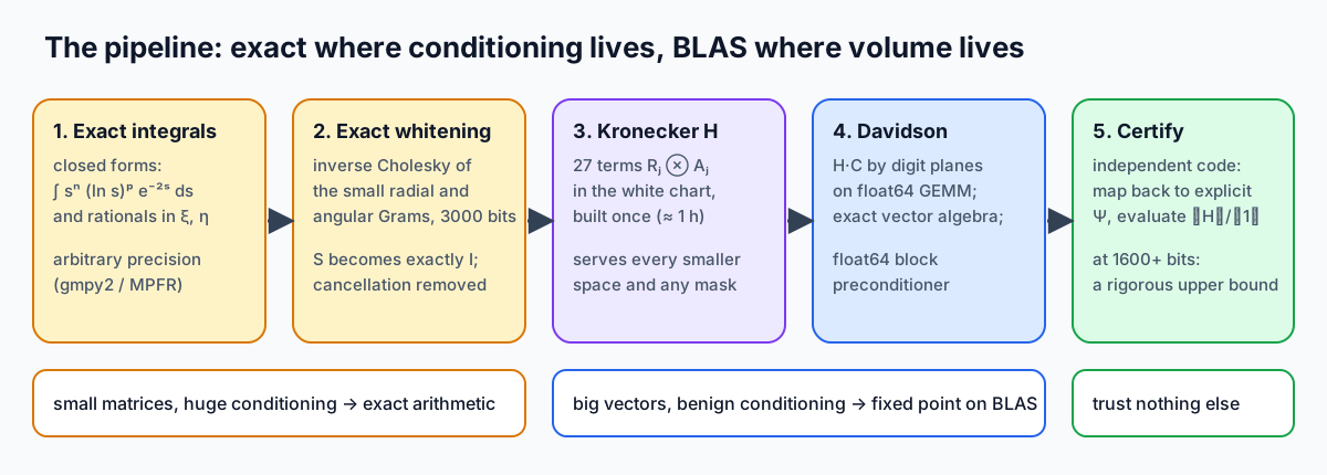The five stages. Amber: exact arbitrary-precision arithmetic, on small objects. Violet and blue: fast arithmetic on large objects. Green: independent verification.

We now navigate through the method one step at a time.

6. The basis: Schwartz’s F-space and a logarithmic tower

We start with Hylleraas coordinates

\[s = r_1 + r_2, \qquad t = r_1 - r_2, \qquad u = r_{12},\]

and a basis that follows Schwartz’s 2006 construction

\[\phi_{lmnp} \;=\; e^{-s}\; s^{\,l}\left(\frac{u}{s}\right)^{m}\left(\frac{t}{s}\right)^{n}(\ln s)^{p}, \qquad l,m\ge 0,\;\; n \text{ even},\;\; p\in\lbrace 0,1\rbrace .\]

Why this particular form? Three reasons.

Homogeneity mirrors Fock. The ratios $u/s$ and $t/s$ are dimensionless and bounded ($0\le u/s\le 1$, $\vert t/s\vert\le1$) so play the role of hyperangles and the power $s^l$ carries the radial scaling. A function with index $l$ is homogeneous of degree $l$ (up to the exponential), which is exactly how the Fock expansion is organised: by powers $R^k$. So $l$ plays the role of $k$.
Negative powers of $s$. Written out, $\phi_{lmnp}\propto s^{\,l-m-n}u^mt^n$, and $l-m-n$ can be negative. Plain Hylleraas bases $s^iu^mt^n$ with $i\ge0$ cannot produce, for example, $u^3/s$, which is homogeneous of degree 2 but not a polynomial. The Fock functions $\varphi_{kp}$ are exactly of this kind
Why $\ln s$ and not $\ln R$. Write $R = s\,g$ with $g = \sqrt{(1+(t/s)^2)/2}\in[1/\sqrt2,1]$. Then $\ln R = \ln s + \ln g$. The $\ln g$ part is a smooth function of the bounded ratio $t/s$ and is represented well by the polynomial angular factors. Only $\ln s$ is singular, so only $\ln s$ needs explicit treatment. (This is also why, in Part III, adding Fock-type $\ln\rho$ functions to a basis that already had radial logs added little.)

Functions are organised into shells $\Omega = l+m+n$. The space $F_\Omega$ contains every function with $l+m+n\le\Omega$ and $p\in\lbrace0,1\rbrace$. Its size is

\[\vert F_\Omega\vert = \sum_{x=0}^{\Omega}\big(\lfloor x/2\rfloor+1\big)\cdot 2\,(\Omega-x+1),\]

where $x = m+n$ is the angular order and the factor $\lfloor x/2\rfloor+1$ counts the even values of $n\le x$. For $\Omega=50$ this is 24,102. Schwartz omits $\ln s$ on shells 0 and 1 (three functions), giving his 24,099.

Note, two indices which are important

the radial degree $l$, the overall power of $s$;
the angular order $x = m+n$, how much structure in $u/s$ and $t/s$ the function carries.

In the isotropic space they are tied together by $l + x \le \Omega$ but we untie them in this work which is one of the most important extensions.

Note, when proofreading this I felt I need to justify/clarify my use of isotropic and anisotropic in this context. I use isotropic to describe the shape of the truncation, meaning the basis treats the two directions of the index grid equally. It is not meant to imply anything physical like it would normally. Each basis function has two indices
$l$, the radial degree (power of $s$)
$x = m + n$, the angular order (how much $u/s$ and $t/s$ structure it carries) What we do is to use different limits in different directions making it anisotropic. We keep the same order Schwartz did, $l + x \le 70$ but also allow $l + x \le 118$ for low angular orders.

The other is to extend $p$ beyond 1, a logarithmic tower $(\ln s)^2,(\ln s)^3$ motivated by the Fock terms $R^4\ln^2R$ and $R^6\ln^3R$.

I attempted a lot of new basis functions which was the original idea of the project. I wanted to develop a new, SOTA basis set which was more compact than those that came before, but I kept running into the same issue whereby promising new basis sets would show good convergence up to 20-30 digits but then hit a hard plateau where the size of the matrix needed to exponentially increase in order to gain the required digits.

My conclusion is that Schwartz’ basis set is highly optimal for these kinds of high accuracy calculations as it is able to maintain convergence for much longer. If I get the time I will write a post on all the different forms I tried and plot their convergence.

7. Box coordinates: turning a wedge into a box

The triangle inequalities of the three particle problem confine $(s,t,u)$ to the wedge $\vert t\vert \le u \le s$. This means that their integral domains are tangled up with each other. Now divide out the scale

\[\xi = \frac{u}{s}\in[0,1], \qquad \eta = \frac{t}{u}\in[-1,1], \qquad\text{so}\qquad u = s\xi,\quad t = s\xi\eta .\]

The Jacobian of $(s,\xi,\eta)\mapsto(s,t,u)$ has determinant of absolute value $s^2\xi$. The weight becomes $W = u(s^2-t^2) = s^3\xi(1-\xi^2\eta^2)$, so luckily the volume element factorises too. The S-state measure $u(s^2-t^2)\,ds\,dt\,du$ becomes

\[u(s^2-t^2)\,ds\,dt\,du \;=\; s^5\,ds\;\cdot\;\xi^2(1-\xi^2\eta^2)\,d\xi\,d\eta .\]

The domain is now a box $[0,\infty)\times[0,1]\times[-1,1]$ which means their integration domains are now independent, and because

\[\left(\frac us\right)^m\left(\frac ts\right)^n = \xi^m(\xi\eta)^n = \xi^{m+n}\eta^n,\]

every basis function is a product of a radial function and an angular function:

\[\phi_{lmnp} = \underbrace{s^{\,l}(\ln s)^{p}e^{-s}}_{f_{lp}(s)}\;\times\;\underbrace{\xi^{x}\eta^{b}}_{g_{xb}(\xi,\eta)}, \qquad x = m+n,\; b = n .\]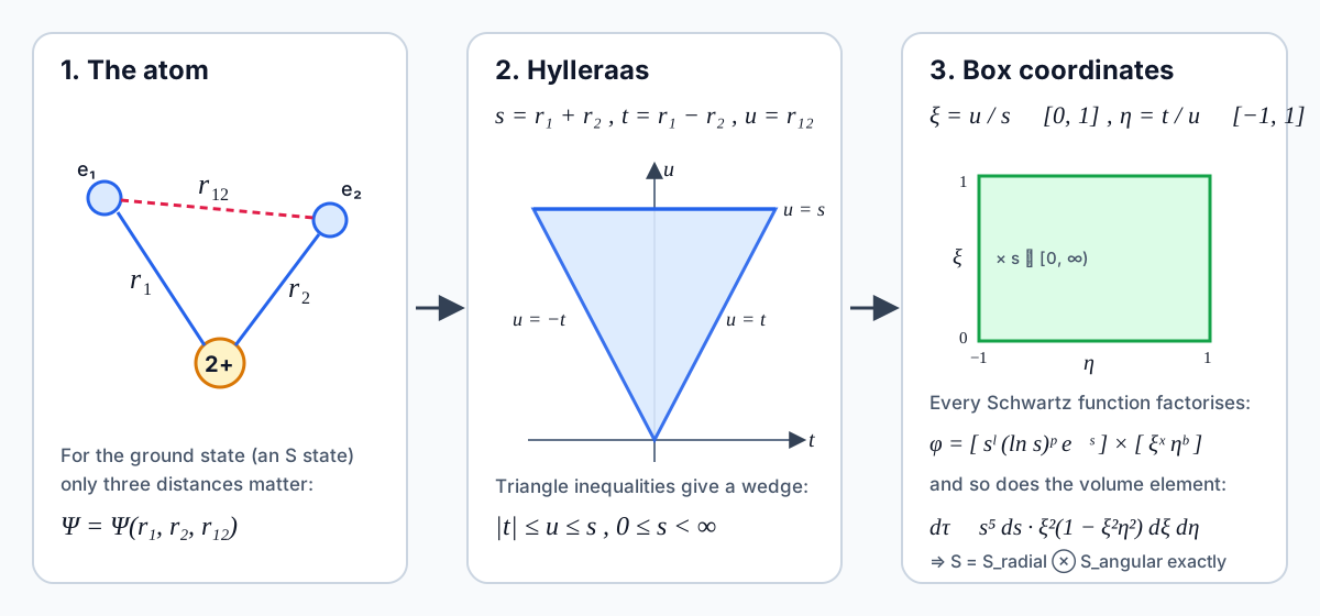

The single change of variables on which everything else rests.

So the overlap matrix is exactly a Kronecker product:

\[\mathbf S = \mathbf S_{\rm rad}\otimes\mathbf S_{\rm ang},\] \[\big(\mathbf S_{\rm rad}\big)_{(l,p),(l',p')} = \int_0^\infty s^{\,l+l'+5}(\ln s)^{p+p'}e^{-2s}\,ds,\] \[\begin{aligned} \big(\mathbf S_{\rm ang}\big)_{(x,b),(x',b')} &= \int_0^1\!\!\int_{-1}^1 \xi^{x+x'+2}(1-\xi^2\eta^2)\,\eta^{b+b'}\,d\eta\,d\xi \\ &= \frac{2}{(b+b'+1)(x+x'+3)} - \frac{2}{(b+b'+3)(x+x'+5)} . \end{aligned}\]

A basis of $N = n_r\times n_a$ functions has an overlap described by one $n_r\times n_r$ and one $n_a\times n_a$ matrix. For the final calculation $n_r\le444$ and $n_a = 1296$, while $N\approx 80{,}000$.

8. The master integrals

Every matrix element of $H$ and $S$ reduces to one family of integrals and the derivative rules below map basis functions to shifted basis functions, and the weights become monomials $s^{d_l}\xi^{d_x}\eta^{d_b}$ in box coordinates. So everything is a sum of master integrals

\[\begin{aligned} K(d_l,d_x,d_b) &= \underbrace{\int_0^\infty s^{\,L+L'+d_l+2}(\ln s)^{P+P'}e^{-2s}\,ds}_{\text{radial}} \\ &\quad\times \underbrace{\frac{1}{X+X'+d_x+2}}_{\int d\xi} \times \underbrace{\frac{2}{B+B'+d_b+1}}_{\int d\eta}, \end{aligned}\]

where the $+2$ in the radial power is the $s^2$ of the Jacobian. The $\eta$ integral vanishes for odd powers, which never occurs in the singlet part.

The radial moments in closed form.

Let $\mathcal R_p(n) = \int_0^\infty s^n(\ln s)^pe^{-as}\,ds$. Differentiating $\int_0^\infty s^{n+\varepsilon}e^{-as}ds = \Gamma(n+1+\varepsilon)/a^{n+1+\varepsilon}$ $p$ times with respect to $\varepsilon$ at $\varepsilon = 0$ gives

\[\mathcal R_0 = \frac{n!}{a^{n+1}}, \qquad \mathcal R_1 = \frac{n!}{a^{n+1}}\big(\psi(n+1)-\ln a\big),\] \[\mathcal R_2 = \frac{n!}{a^{n+1}}\Big[\big(\psi(n+1)-\ln a\big)^2 + \psi'(n+1)\Big],\]

and in general $\mathcal R_p = \frac{n!}{a^{n+1}}\,B_p(\kappa_1,\dots,\kappa_p)$, a complete Bell polynomial in $\kappa_1 = \psi(n+1)-\ln a$ and $\kappa_j = \psi^{(j-1)}(n+1)$ for $j\ge2$. At integer arguments the polygamma functions are harmonic-type sums

\[\psi(n+1) = H_n - \gamma, \qquad \psi^{(m)}(n+1) = (-1)^{m+1}m!\,\Big(\zeta(m+1) - \sum_{k=1}^n k^{-(m+1)}\Big).\]

So everything is a rational number, $\gamma$, $\ln 2$ and $\zeta$-values, all computable to any precision.

9. Derivatives, and why there are exactly 27 terms

To use the functional of §4 we need $\partial_s$, $\partial_t$, $\partial_u$ in box coordinates. At fixed $t,u$, $\xi = u/s$ depends on $s$ but $\eta = t/u$ does not; at fixed $s,u$ only $\eta$ depends on $t$; at fixed $s,t$ both $\xi$ and $\eta$ depend on $u$. Using our friend the chain rule

\[\begin{aligned} \partial_s &= \partial_s^{\rm rad}\otimes I \;-\; s^{-1}\otimes \xi\partial_\xi, \\ \partial_t &= s^{-1}\otimes \xi^{-1}\partial_\eta, \\ \partial_u &= s^{-1}\otimes \xi^{-1}\big(\xi\partial_\xi - \eta\partial_\eta\big). \end{aligned}\]

Acting on basis functions these are index shifts

\[\begin{aligned} \partial_s^{\rm rad}\big[s^L(\ln s)^Pe^{-s}\big] &= L\,s^{L-1}(\ln s)^P + P\,s^{L-1}(\ln s)^{P-1} - s^L(\ln s)^P,\\ \xi\partial_\xi\,\big[\xi^X\eta^B\big] &= X\,\xi^X\eta^B,\\ \xi^{-1}\partial_\eta\,\big[\xi^X\eta^B\big] &= B\,\xi^{X-1}\eta^{B-1},\\ \xi^{-1}(\xi\partial_\xi-\eta\partial_\eta)\,\big[\xi^X\eta^B\big] &= (X-B)\,\xi^{X-1}\eta^{B}. \end{aligned}\]

Each derivative is a short sum of (radial operator) ⊗ (angular operator), which I refer to as a bank; the value has 1 term, $\partial_s$ has 2, and $\partial_t$ and $\partial_u$ have 1 each. The weights of §4 in box coordinates become

weight	in $(s,t,u)$	as box monomials $s^{d_l}\xi^{d_x}\eta^{d_b}$
overlap / $\Psi_s^2,\Psi_t^2,\Psi_u^2$	$u(s^2-t^2)$	$s^3\xi - s^3\xi^3\eta^2$
$\Psi_s\Psi_u$ cross term	$s(u^2-t^2)$	$s^3\xi^2 - s^3\xi^2\eta^2$
$\Psi_t\Psi_u$ cross term	$t(s^2-u^2)$	$s^3\xi\eta - s^3\xi^3\eta$
potential	$s^2-t^2-4Zsu$	$s^2 - s^2\xi^2\eta^2 - 4Z\,s^2\xi$

Lets count the (bra bank) × (weight monomial) × (ket bank) products

$\Psi_s^2$: $2\times2\times2 = 8$;
$\Psi_t^2$ and $\Psi_u^2$: $2+2$;
the two $\Psi_s\Psi_u$ orderings: $4+4$;
the two $\Psi_t\Psi_u$ orderings: $2+2$;
potential: $3$.

This totals 27 terms, and each is a Kronecker product

\[\mathbf H \;=\; \sum_{j=1}^{27} c_j\; \mathbf R_j\otimes\mathbf A_j .\]

Only 6 distinct radial matrices and 26 distinct angular matrices appear. Terms that share an angular matrix can be merged on the radial side, $\mathbf M_A = \sum_{j:\mathbf A_j = A} c_j\mathbf R_j$.

Something which I knew would be mandatory at the start of this project is the ability to apply H without forming it. as the matrices needed for this eigenvalue problem would take considerable storage space in RAM. Rough estimates place a 80,000 x 80,000 dense matrix of 128 digit numbers as ~ 414GB which far exceeds the 24GB of the MacBook! Using the Kronecker factors we only need 2.9GB which can be stored easily with room to spare.

To do this we store the coefficients as a grid $\mathbf C$ with rows indexed by radial functions $(l,p)$ and columns by angular functions $(x,b)$. The identity $(\mathbf R\otimes\mathbf A)\,\mathrm{vec}(\mathbf C) = \mathrm{vec}(\mathbf R\,\mathbf C\,\mathbf A^{\mathsf T})$ gives

\[\mathbf H\,\mathbf C = \sum_{A}\mathbf M_A\,\big(\mathbf C\,\mathbf A^{\mathsf T}\big),\]

which is two dense matrix–matrix products per distinct angular matrix; Some quick NumPy code brings it to life

  
def apply_H(C, parts):                  # C: (n_r, n_a) coefficient grid
    return sum(M @ (C @ A.T) for A, M in parts)   # 26 pairs (A, M_A)

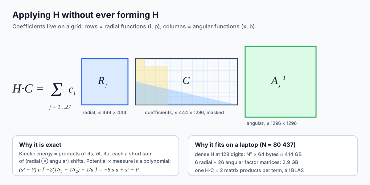For N = 80,437 a dense H at 128-digit precision would need about 414 GB; the Kronecker factors need 2.9 GB.

The truncation $l+x\le\Omega$ is just a statement about which grid entries may be non-zero. If we apply $\mathbf H$ to the full grid and zero the entries outside the mask afterwards, that is exactly the projection onto the chosen subspace. Any mask costs the same, which frees the shape of the variational space from the shape of the Schwartz shell (§12).

10. Exact whitening

I have used whitening routinely over the years as a means of converting a severely ill-conditioned generalised eigenvalue problem into a standard symmetric eigenvalue problem by orthonormalising the underlying basis. It allows us to isolate and localise the ill conditioning into a set of much smaller matrices which we can then focus all our numerical firepower on, without needing to run the entire calculation at very high precision.

In this case the raw basis is catastrophically non-orthogonal, at order 32, the transformation to an orthonormal basis already has entries around $10^{26}$. At order 56 the cancellation depth is about 90 decimal digits, and with the $(\ln s)^3$ functions included the radial Gram’s Cholesky factorisation fails at 2000 bits (~ 600 digits, six hundred, 6-0-0, ridiculous). Solving $\mathbf Hc = E\mathbf Sc$ directly in such a basis is hopeless in any fixed precision.

The massive benefit of the Kronecker structure we have developed and the reason it makes up part of the methods acronym, is that it makes the solution to this much cheaper. We compute the inverse Cholesky factors of the two small Grams

\[\mathbf S_{\rm rad} = \mathbf L_r\mathbf L_r^{\mathsf T},\quad \mathbf U_r = \mathbf L_r^{-\mathsf T}; \qquad \mathbf S_{\rm ang} = \mathbf L_a\mathbf L_a^{\mathsf T},\quad \mathbf U_a = \mathbf L_a^{-\mathsf T},\]

in exact arbitrary-precision arithmetic (gmpy2/MPFR at 3000 bits). Then transform every factor once

\[\mathbf R_j \leftarrow \mathbf U_r^{\mathsf T}\mathbf R_j\mathbf U_r, \qquad \mathbf A_j \leftarrow \mathbf U_a^{\mathsf T}\mathbf A_j\mathbf U_a .\]

In this white chart, $\mathbf S = \mathbf I$ and the problem is the ordinary symmetric eigenproblem $\mathbf H\mathbf c = E\mathbf c$

The cancellation is removed. A white matrix element is $\langle w_i\vert O\vert w_j\rangle$ between orthonormal functions. Its size is controlled by the operator (large for high-kinetic-energy functions, but never the result of cancelling $10^{90}$-sized terms). All the cancellation happened inside the exact factorisation, where it was harmless, and each white matrix element is stored as a sum of eight doubles (about $10^{-67}$ relative)
Graded invariance. Cholesky is triangular and if the functions are ordered so that every smaller space is a prefix of the ordering, the first $k$ white functions depend only on the first $k$ raw functions. Then one build at the largest order serves every smaller order and every mask that is a prefix in each row and column. The radial ordering is $(l,p)$ with $p\le1$ interleaved by $l$ up to $l = 120$, then all $p = 2$ rows, then the $p = 3$ rows. The angular ordering is by $x$, then $b$
A subtlety for the log tower. A white $(\ln s)^2$ function is orthogonalised against all $p\le1$ radial functions up to $l = 120$, including ones outside a given mask. So in a masked space the white log functions carry small components of raw functions the mask excludes. This is harmless: any subspace gives an upper bound, and the certifier evaluates exactly the function the white coefficients describe. But it means a coefficient vector cannot be moved between two builds with different radial orderings just by matching labels. That cost me real time in the final push (Chapter 8)

The whitening is the central trade of the method: the ill-conditioning never goes away, but it is moved into two matrices of at most 1,296 rows, computed exactly, once, in under an hour. I think this was the most important breakthrough of the project as this was a wall I kept routinely hitting from every angle of attack I developed.

11. 280-bit arithmetic at the speed of float64 BLAS

This section contained one of the biggest learnings for me. In the white chart, fixed-point arithmetic is enough. The remaining problem is speed; the $H\,C$ products must be accurate to ~$10^{-67}$ and run at hardware speed because we are only using a laptop. I have written previously on using DoubleDouble and QuadDouble datatypes for fast, high accuracy calculations which I learned from the work of David Bailey. For this project I implemented and optimised my own OctDouble datatype using these principles but even though it was much faster than equivalent MPFR types, it was still a significant computational bottleneck.

In the white chart, fixed-point arithmetic suffices. The coefficient vector is stored as integers at scale $2^{-280}$ (absolute resolution about $5\times10^{-85}$). The remaining question is speed. A software multiprecision matrix product is 100–1000 times slower than hardware BLAS, and $\mathbf H\mathbf C$ is about $2\times10^{10}$ multiply–adds.

I hit the books (research papers?) and came across a very useful trick error-free splitting, known as the Ozaki scheme which I attempt to now do justice to

Normalise. Scale each row of each operand by a power of two so that its largest entry uses exactly 294 bits
Slice. Write every entry as $x = \sum_{s=0}^{13}x_s\,2^{-21s}$ with $\vert x_s\vert < 2^{21}$. Each slice is a small integer, stored exactly in a float64 (incredibly useful!)
Multiply slices exactly. A slice product summed over $k$ terms is bounded by $2^{21}\cdot2^{21}\cdot k$. For $k\le2^{11}$ this is at most $2^{53}$, so an ordinary float64 GEMM computes it exactly, with no rounding at all. Our inner dimensions are at most 1,296
Skip what cannot matter. The product of slices $s$ and $t$ has weight $2^{-21(s+t)}$ relative to the leading term. Pairs with $s+t>13$ contribute below $2^{-220}$ relative and are dropped
Recombine exactly. Convert each GEMM result to int64, group by $s+t$, and combine the groups with exact integer shifts. Then undo the row scalings

  
def slices(X_int, beta=21, planes=14):            # X_int: row-normalised integers (object array)
    sign, mag = np.sign(X_int), np.abs(X_int)
    return [sign * ((mag >> (beta * (planes - 1 - s))) & ((1 << beta) - 1)) for s in range(planes)]
# product: sum over s + t <= 13 of  float64 GEMM(slice_s(X), slice_t(M).T)  -- each exact

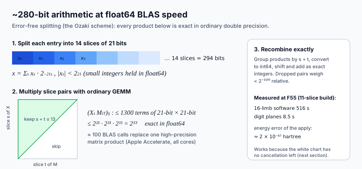About a hundred ordinary BLAS calls replace one high-precision matrix product, all on Apple Accelerate across every core.

The effect was very dramatic and allowed for iteration on all these ideas much faster. At $F_{55}$ a full $\mathbf H\mathbf C$ took 516 s in 16-limb software floating point (C++, all cores) and 8.5 s using digit planes and the Ozaki scheme, with the energy exact to $2\times10^{-67}$. That measurement was with an earlier 11-slice version; the production version uses 14 slices for a bit more headroom.

I will be using this idea in other projects moving forward as it is elegant and very effective.

12. Choosing the space: measure first

I think this is primarily where the extra digits came from and where I ended up wasting substantial time. Climbing the isotropic Schwartz ladder $F_{50}\to F_{62}$ with the machinery above gave diminishing returns: 12 more shells and 20,000 more functions bought fewer than 4 digits. After a lot of attempts at incremental improvements (am I Codex or Claude?) I stopped adding functions and measured where the missing energy was actually located

The isotropic ladder stalls. With the machinery above, climbing $F_{50}\to F_{62}$ was straightforward. But the gain per two orders, which for a long time fell by a steady factor of about 40, suddenly collapsed.

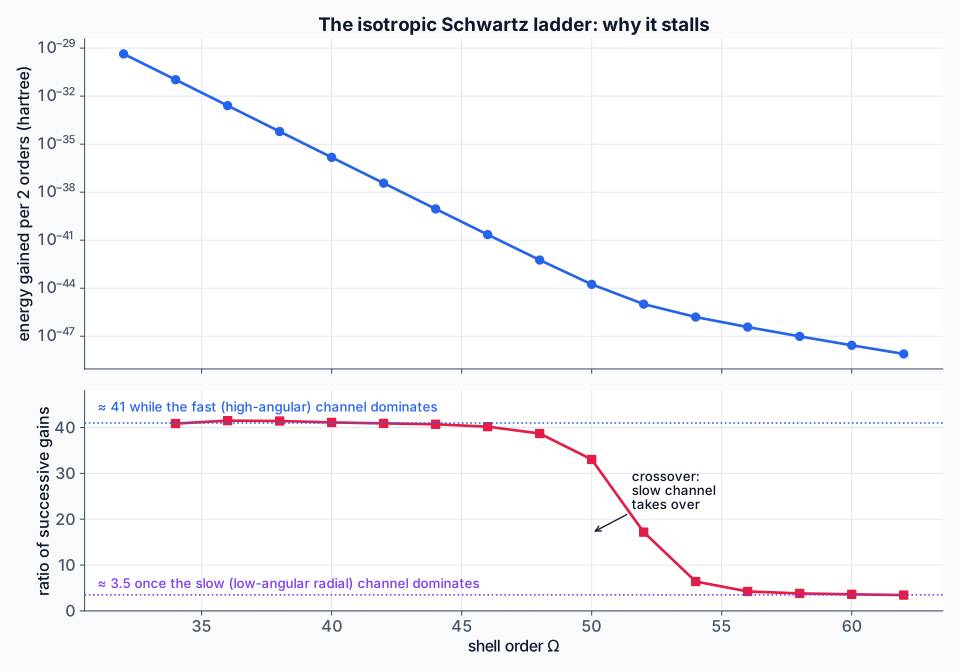The ratio of successive gains drops from about 40 to about 3.5 within eight orders. That is not what a single convergence rate looks like.

There is a lot going on in this plot so lets break it down. The top panel is the energy gained each time two more shells are added to Schwartz’s basis, on a log scale. The bottom panel is the ratio between successive gains, which measures how fast the calculation is converging.

Up to about $\Omega = 46$ the convergence is consistent with each pair of shells gaining about 41 times less than the one before; a perfectly steady ratio, so the energy converges geometrically and digits lock-in at a constant rate. Then, between $\Omega = 48$ and $56$, the ratio collapses: $39$, $33$, $17$, $6.4$, then $4.2$, finally settling at about $3.5$. From there each new pair of shells, thousands of extra functions, buys only a few times less than the last. Going from $F_{50}$ to $F_{62}$ adds 20,000 functions but fewer than four digits.

It stalls because a single convergence rate can’t produce that shape, but two can. The wavefunction has two kinds of structure converging at very different speeds

High-angular structure (lots of $u/s$ and $t/s$ dependence) converges fast: about 37 times per two orders
Low-angular structure with high radial degree (high powers of $s$, where Fock’s logarithms live) converges slowly: only about 4 times per two orders

Early on, the fast part dominates the error, so the ladder converges fast. But its error shrinks so quickly that around $\Omega \approx 48$ the slow part overtakes it, and from then on the slow part sets the pace.

The deeper cause is the shape of Schwartz’s basis. The rule $l + x \le \Omega$ gives radial degree and angular order a single shared budget, so each new shell spends most of its functions on angular structure that is already converged and only a few on the radial structure that is starving. This was my cue to change the shape rather than the size; add radial degree only at low angular order. The same $4\%$ more functions then cut the remaining error by a factor of 460,000.

A two-parameter model

\[\Delta E(\Omega) \approx a\,w_{\rm fast}(\Omega) + b\,w_{\rm slow}(\Omega)\]

reproduces the whole $F_{46}$–$F_{54}$ ladder to 3%. At low $\Omega$ the fast channel dominates and the ladder converges at the fast rate. Near $\Omega\approx48$ the slowly converging low-angular channel overtakes it, and from then on the ladder converges at the slow rate. The measured ratios settle at about 3.5 by $\Omega = 62$, consistent with that picture.

I also ran independent localisation experiments which showed the same thing. An exact Rayleigh–Ritz step from $F_{55}$ into candidate function sets showed the missing energy concentrated at high radial degree and low angular order. Adding about 300 such functions lowered the energy by $1.7\times10^{-47}$, against $3.2\times10^{-52}$ for 300 extra angular functions, and about $10^{-55}$ for functions with a second exponential scale (independent of that scale).

The consequence is that the isotropic shell $l+x\le\Omega$ is the wrong shape. It raises the radial degree of every angular channel together, spending thousands of functions on high-angular channels that are already converged, while the low-angular channels starve. The masks of §9 fix that for free. Raise the radial degree only where it is needed:

\[\text{keep } l + x \le \Omega_{\rm ang} \text{ for all } x, \quad\text{and allow } l + x \le \Omega_{\rm rad} \text{ for } x < x_{\rm cut}.\]

The gain is out of all proportion to the cost. At $\Omega_{\rm ang}=62$, extending the radial degree to 90 for $x<10$ adds 1,680 functions (4%) and lowers the energy by $3.5\times10^{-49}$, more than the entire last isotropic shell (2,048 functions). The remaining error of $F_{62}$ falls from $3.5\times10^{-49}$ to $7.6\times10^{-55}$, a factor of about 460,000.

We can see now that the log series is closing fast, exactly as Fock’s expansion suggests, which leads us onto what I call the log tower (I am a fan of the science fiction writer Ted Chiang and I picture this log tower the way he describes it in his short story, “The tower of Babylon” for some reason. I do not think this has any relevance at all, I just wanted to share it).

Fock’s expansion puts $(\ln R)^p$ with $R^{k}$, $p\le k/2$. The natural rule would be to add $(\ln s)^2$ only for radial degree $l\ge 4$ and, since the Fock structure lives in low angular channels, only for small $x$. I tested both. Allowing $(\ln s)^2$ for all $l$ and for $x<20$ beat the Fock-rule version ($l\ge4$, $x<10$) by $2.1\times10^{-55}$. In a truncated basis the log functions also help represent structure the rule does not anticipate. The $(\ln s)^2$ tower is worth $5.1\times10^{-55}$ in total, and the $(\ln s)^3$ tower (capped at $l\le80$ for conditioning) $4.2\times10^{-62}$. The drop of seven orders of magnitude from one log power to the next is the clearest sign that the log series has converged.

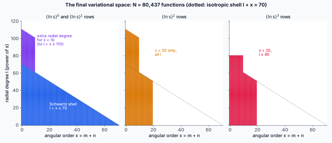The largest space used, N = 80,437. Every coloured cell is one or more basis functions; the dotted line is the isotropic shell. The best bound in Part IV uses the same angular shell with the radial degree raised to 118 and the (ln s)² tower (N = 74,247).

Each panel in this is a map of which basis functions are in the final variational space.

The horizontal axis is the angular order $x$: how much dependence on the electron–electron distance and on $(r_1 − r_2)$ a function carries
The vertical axis is the radial degree $l$, the power of $s = r_1 + r_2$, which describes how the wavefunction varies with overall size
Every coloured cell is a group of basis functions at that $(l, x)$
The three panels are the same map for functions multiplied by different powers of $\ln s$.
The dotted diagonal, $l + x = 70$, is the edge of Schwartz’s standard basis

Left panel: ordinary functions, $(\ln s)^0$ and $(\ln s)^1$. The blue triangle is Schwartz’s shell, everything with $l + x \le 70$, which is 63,492 functions. The violet strip on top is the extra radial degree, added only for low angular order $(x < 10)$, up to $l + x \le 110$. It is only 2,400 functions, about $4\%$ of the space. These are exactly the high-power, low-angular functions the convergence analysis said were missing, and they do most of the work beyond Schwartz.

Middle panel: the $(\ln s)^2$ tower, 7,635 functions. Fock showed that where both electrons meet the nucleus, the exact wavefunction contains logarithms, starting with $R^2$ $\ln R$ and then $R^4$ $(\ln R)^2$. Ordinary powers can only imitate these slowly, so we add them explicitly. They are only needed at low angular order, so the tower stops at $x < 20$. It follows the same radial limits as the left panel: the extended strip for $x < 10$, and the Schwartz edge above it.

Right panel: the $(\ln s)^3$ tower, 6,910 functions, the next term in Fock’s series. It covers the same angular range but stops at $l = 80$. Beyond that, these functions become so nearly identical to the lower log powers that even 2,000-bit arithmetic cannot tell them apart.

The shape is telling us that the Schwartz’s basis is a triangle; every direction grows at the same rate but ours is lopsided on purpose. It spends extra functions only where measured convergence was slow, on high radial degree and logarithms at low angular order, and leaves the fast-converging high-angular region alone.

The log tower also shows that it has converged. $(\ln s)^2$ lowered the energy by $5 × 10^{-55}$; $(\ln s)^3$ by only $4 × 10^{-62}$, seven orders of magnitude less!

13. Solving: Davidson in the white chart

Here comes another learning. In the white chart the problem is a standard symmetric eigenproblem for the lowest eigenvalue. I was previously aware of the Krylov subspace method but for this project learned about the Davidson solver which is an iterative, projection-based version of the Krylov method. I had heard mention of the Davidson solver before, but had never actually implemented or used it before

Project. Update the $k\times k$ matrix $G_{ij} = v_i\cdot h_j$. Only the new row is computed each iteration; the rest is cached.
Solve small. Find the lowest eigenpair $(\theta, y)$ of $G$ in 110-digit arithmetic.
Ritz vector and residual. $x = \sum y_iv_i$, $\mathbf Hx = \sum y_ih_i$, $r = \mathbf Hx-\theta x$, all exact.
Correct. Approximately solve the correction equation $(\mathbf H-\theta)\,t = -r$ with a preconditioner $M\approx \mathbf H-\theta$, i.e. $t = -M^{-1}r$.
Expand. Orthogonalise $t$ against the basis (twice, exactly), normalise, apply $\mathbf H$, and append.

Residual versus energy. The energy error of a Ritz value is roughly $\sum_i r_i^2/(\lambda_i-\theta)$, summed over eigen-directions. Components of the residual along high-energy directions (large $\lambda_i$) cost almost nothing in energy. That is why a residual norm of $10^{-25}$ is compatible with an energy converged to $10^{-62}$ as most of the residual lives in directions with $\lambda_i$ up to $10^{14}$. It is also why a Temple-type lower bound built from $\Vert r\Vert^2$ alone would be useless here.

I then fell into another trap which cost me days.

The preconditioner: block-exact, merged sectors. $M$ is block-diagonal. Each block is the exact restriction of $\mathbf H$ to a group of angular-order sectors, assembled in float64 from the 27 Kronecker terms and factored once. In a first version each block was a single angular order $x$, which ignores all coupling between neighbouring orders. Merging neighbouring sectors into blocks of up to 8,000 functions made the preconditioner see that coupling, and cut iterations 2.5-fold at $F_{30}$. At $F_{56}$ it reached residual $1.6\times10^{-28}$, with the energy settled to $10^{-63}$, in 40 iterations; per-sector blocks were still at $3\times10^{-23}$ after 40.

The float64 trap. The whitened log functions have enormous kinetic energies. Their diagonal elements reach $10^{14}$, and the blocks containing them have norms around $10^{18}$. Assembled in float64, every entry carries a relative rounding error of about $\epsilon\approx10^{-16}$. For a symmetric positive-definite matrix, $\vert H_{ij}\vert\le\sqrt{H_{ii}H_{jj}}$. So in the diagonally scaled matrix $D^{-1/2}HD^{-1/2}$ ($D = \mathrm{diag}\,H$) the rounding perturbation has norm at most about $n c\,\epsilon$, where $n$ is the block size and $c$ the number of summed terms. That is small relative to the scaled matrix but enormous relative to the physically important small eigenvalues.

In practice the assembled blocks had eigenvalues near $-800$. That is impossible for a sub-block of a Hamiltonian whose lowest eigenvalue is $-2.9$. With those blocks both eigh and Cholesky gave garbage, the corrections pointed the wrong way, and the solver stalled at a residual of $10^{-21}$. The fix is a diagonal shift of the size of the rounding perturbation:

\[M_b = H_b - \theta I + \tau\,\mathrm{diag}(H_b), \qquad \tau = 10^{-12},\]

factored by Cholesky (with $\tau$ escalated from 0 only on the blocks that need it). The shift moves the physically important low-$l$ rows (diagonal $\sim1$–$10^3$) by only $10^{-12}$–$10^{-9}$, far below their gaps of $\sim10^{-2}$. The iteration after this fix gained more energy than the previous forty combined!

Other details that mattered.

Olsen’s correction which replaces $-M^{-1}r$ by $-M^{-1}r + \varepsilon M^{-1}x$ with $\varepsilon = (x\cdot M^{-1}r)/(x\cdot M^{-1}x)$, to stop the correction collapsing onto the current Ritz vector.
Thick restart. When the subspace reaches 60 vectors, we restart with the Ritz vector plus the last 10 basis vectors (their $\mathbf H$-products are already known, so no new applies are needed). This keeps the recent Krylov information.
Continuation. Each space is seeded from the solution in the previous, smaller space. The correction from one rung to the next is tiny in energy ($10^{-55}$) but spread collectively over tens of thousands of coefficients, and a good seed is worth hundreds of iterations. Seeds must come from the same whitened build (§10).
Stopping. Stop when the residual is below target, or after three consecutive (non-restart) energy changes below $10^{-64}$, or at an iteration cap. The final tail of energy changes is recorded and becomes a line in the error budget.

14. Certification: trust nothing else

I learned this lesson the hard way from a previous, related project. The solver’s number is not the result. We need to certifiy using a separate program that shares no code with the solver

Map the white coefficients back to explicit Schwartz monomials, $\mathbf M = \mathbf U_r\mathbf C\mathbf U_a^{\mathsf T}$, giving $\Psi = \sum c_{lmnp}\phi_{lmnp}$ as an explicit function
Recompute the whitening factors independently from the closed-form Grams
Evaluate $\mathcal N[\Psi]$ and $\mathcal D[\Psi]$ of §4 directly, in box coordinates, from the master integrals, at 1600+ bits

Because $\Psi$ is explicit, $\mathcal N/\mathcal D$ is a rigorous upper bound, up to arithmetic error below $10^{-80}$. For every state in this post, solver and certifier agree to between $10^{-74}$ and $10^{-84}$, and $\Vert\Psi\Vert^2-1$ is below $10^{-84}$.

Another useful quality of a certifier is that it can act as a bug detector. It exposed a native 128-bit code path whose “energies” were $4\times10^{-51}$ below the true Rayleigh quotient of the function they described, which is not a valid bound at all (Chapter 6).

Part III: The road to the solution

If you think I have rambled enough already you aint seen nothing yet. Feel free to log off and question the time you have spent reading this thus far if you have made it here.

The description in Part II makes it look like I developed the method in this methodical order; it was not so. This is the order in which things actually happened and what each step taught. I went down many incorrect avenues and made many mistakes before realising the correct path to take. The ground rules from the start were

the calculation must actually run on my MacBook
the method should not be a reimplementation of another author
ideally, the basis should be compact, giving more digits per basis function than anyone else

I achieved the first two goals but not the third. These following sections are some of the important developments, what the results were and more importantly what I learned from them.

Chapter 1: Precision is a gate

The first code I developed was a Hylleraas-type basis with an extra exponential-integral term $E_1(\beta s)$ (which carries a logarithm and a second length scale). It was solved in double-double arithmetic (about 32 digits).

It hit a wall at shell order $\Omega\approx14$, about 13.5 digits, which I thought was the basis. It turned out that the difference between double-double and quad-double energies grew by roughly ×300 per shell, because the overlap’s condition number grows like $10^{1.6\,\Omega}$. Past $\Omega\approx13$, adding functions made the double-double answer worse.

So I built an oct-double backend: numbers as unevaluated sums of eight doubles, 424 bits, about 126 digits. It used the CAMPARY library, plus my own exp and log (weirdly CAMPARY has none) and the numeric-limits plumbing needed to run Eigen’s symmetric eigensolvers in that type. I validated it against mpmath to 124–126 digits.

Lesson. If a convergence series decelerates when you add functions, check the arithmetic before the physics. Run the same calculation at two precisions; if they diverge, you are measuring rounding not basis error.

Chapter 2: What actually moves the convergence slope

With precision out of the way, I ran a systematic set of low-order basis experiments. Most were negative, but I learned from each one

More exponential scales do not help. At equal basis size, multi-scale bases were no better, and the optimiser drove the scale ratios towards 1. Extra scales just shifted the digits-versus-$N$ curve to the right
Explicit $(\ln s)$ looked worse than $E_1$ at low order. At $N = 322$, polynomial + $\ln s$ gave 8.8 digits against 11.7 for polynomial + $E_1$. This was a misleading negative as low order $E_1$ wins because of its second length scale, not its logarithm. At high order (Part II) explicit logs are indispensable, low-order evidence about asymptotic structure is weak evidence
A correlation factor $e^{-\gamma u}$ (Korobov-style) shifted the fixed-$\Omega$ wall: at $\Omega=6$, 9.1 → 10.3 digits, but unfortunately it was an offset, not a new slope
Transcorrelation (move $e^{\gamma u}$ into a non-Hermitian similarity-transformed Hamiltonian) gave exactly the same slope (0.377 vs 0.387 digits per order) and lost the variational bound. In Hylleraas coordinates the linear $u$ term already captures the electron–electron cusp, so there is nothing for transcorrelation to win
An explicit Fock sector (functions $\rho$, $\ln\rho$, $\rho\ln\rho$ times Hylleraas polynomials, with $\rho$ the hyperradius) doubled the slope, from 0.70 to 1.37 digits per order. This was the first lever that changed the slope rather than the offset. It confirmed that the wall is the non-analytic triple-coalescence structure
The Fock sector subsumes $E_1$. Since $\ln\rho = \ln s + \ln g$, the Fock generators already contain the radial log that $E_1$ provides, plus an angular part $E_1$ cannot. Adding $E_1$ on top of Fock gained only +0.1 digit

I derived closed-form Fock kernels and ported them to C++ in oct-double, gating every step. Angular and radial kernels were checked to 121–124 digits, whole matrices element by element against the Python reference, and end-to-end energies against the prototype.

The most useful learning: the second-derivative kinetic operator is non-Hermitian by a boundary term for log-singular functions. That is why the final method uses the gradient form (§4) exclusively.

Lesson. Measure slopes, not offsets. Almost every idea improved the energy at fixed order; almost none changed the rate at which digits accumulate. Only the rate matters for a record such as this

Chapter 3: The solve wall, and my dream of compactness shattered

With a good basis, the bottleneck became the dense oct-double eigensolve. It scales as $O(N^3)$: 9.5 s at $\Omega=8$, 1,750 s at $\Omega=10$. Memory scales as $O(N^2)$ times 8 limbs: an estimated 180 GB at $\Omega=28$.

The obvious fixes failed, and I measured each one

a precision ladder (solve low orders in lower precision) was slower, because lower precisions fell back to a general non-symmetric solver
a mixed-precision factorisation with fewer limbs stalled inverse iteration and fell back to the full solver, 20 times slower
orthogonalising away near-dependencies bought little progress. The condition number is floored by the accuracy target itself, roughly $10^{2.4\,\times\,\text{digits}}$, so at 25 digits the basis still needs a condition number around $10^{60}$

One of the motivations for wanting a compact basis is to avoid heading into the territory of ill conditionin, i.e., if the basis cannot be conditioned better, make it smaller. This became a long, productive and ultimately bounded pathway

A response-contraction method compressed Schwartz-type functions into a few hundred contracted directions
A “Change D” rewrite evaluated each of the 2,186 globally distinct monomials once instead of per column, 15× less integral work
The Fock generators were integrated into the compressed builder

Chapter 4: The era of searching for a compact-basis, and the three-wall pattern

For weeks the goal was a compact record: fewer explicit functions than anyone for the same accuracy. I tried a long list of ideas:

Approach	Best result	Why it stopped
Korobov-style correlated exponentials, greedy Sobol + Nelder–Mead growth	8.1 digits at N = 41	slope collapsed to 0.06 digits per function; a single addition took 13 min
Bayesian optimisation of the exponents	5.00 vs 5.09 digits for random search	the per-step search is 3-D; acquisition was not the bottleneck
Homotopy residual pursuit (switch on $1/r_{12}$ gradually, grow atoms along the path)	beat a direct run by 0.38 digits at N = 20	the macro loop is a convergent series: each teacher offered a constant ~0.4 digits but the retained fraction decayed (0.81 → 0.64 → 0.37), capping at 11–12 digits
Response envelopes (one nonlinear centre, several linear channels), fixed-size surgery, pruning	crossed 10 and 11 digits with a few hundred directions	slope decayed
Riccati–Fock minimax, complex exponents, signed packets	isolated positive gates	never decisive at matched size
Rational / multidomain Galerkin (FRT-RG, FAM-RG, FF-VPS)	positive gates	convergence not strong enough
Continuous (fractional) Fock orders	+0.02 digits over integer orders	conditioning-fragile; the integer ladder is the asset
General correlated Fock kernel, $\rho^k(\ln\rho)^p e^{-As-Bt+Cu}$	validated to $10^{-13}$; +0.8 digits even with correlation	a real kernel, but on top of a machinery already at its ceiling

Taken together, these showed a three-wall pattern. Every compact machinery hit a ceiling (around 8 digits for greedy exponentials, 11–12 for the macro loop). The Schwartz-type space kept converging, but slowly and expensively. The ceilings were not bugs in the code or method they were the structure of the approach itself.

Lesson. A method with a decaying digits-per-function curve has a finite ceiling, and you can estimate it early by fitting the decay. Doing that saved weeks each time I did it, and cost weeks each time I did not.

Chapter 5: FLAKE, the pivot to a big orthogonal space

The pivot was to give up compactness and ask a different question: can the full Schwartz $F_\Omega$ ladder be pushed past order 50 on a laptop? That required three changes:

orthogonalise the space, so the eigensolver never sees the overlap’s condition number;
apply $H$ matrix-free in oct-double, so memory is $O(N)$;
solve with Davidson, seeding each order from the last.

Low orders behaved perfectly: $F_{10}$, $F_{12}$, $F_{14}$ converged with an almost flat number of Davidson vectors (66, 60, 66). Then three episodes shaped everything after.

The false alarm. A first $F_{30}\to F_{40}$ attempt appeared to stall $10^{-25}$ above Schwartz’s value so I thought the implementation was broken. In fact the comparison target was wrong and the $F_{30}$ state was under-converged. After a correct fixed-space solve, $F_{30}$ matched Schwartz’s $F_{30}$ to $9.8\times10^{-34}$ with residual $1.8\times10^{-14}$.

The collective correction. Jumping from $F_{30}$ straight to $F_{40}$ (7,070 new functions) failed. I tried single-vector Davidson, sector blocks, raw residual directions, MINRES, GMRES and short Lanczos spaces; the best moved about 0.8% of the known correction. The missing energy was in the space, but spread collectively across thousands of coefficients. The fix was a staircase, $F_{30}\to F_{32}\to F_{34}\to\cdots$, each rung seeded by the last.

The corrupt preconditioner. At $F_{32}$ the residual floored at $1.8\times10^{-13}$, in both double-double and quad-double preconditioner builds. The cause was cancellation in building the preconditioner blocks: one diagonal element whose true value was 7,411 came out as 793.5. Building the tail block column by column with the trusted oct-double operator broke the floor immediately. The full oct-double preconditioner then converged $F_{32}$ to residual $9.6\times10^{-17}$, landing exactly on the fitted convergence line at 31.4 digits. But that build took 4.3 hours, against 9 minutes for the solve. (A cheaper double-double-core / oct-double-tail hybrid failed the same gate.)

The staircase climbed to $F_{55}$ (31,668 functions). Our $F_{50}$ matched Schwartz’s to $4.8\times10^{-47}$ (our space has his three missing functions), and $F_{52}$ went clearly below his value. Then the convergence stalled.

Lesson. Before concluding a method fails, check the target, and check the approximate components. Both of the “method failures” in this chapter were a wrong reference and a corrupt preconditioner. The exact operator was right all along.

Chapter 6: The F55 wall, and an audit for validation

Between $F_{50}$ and $F_{55}$ the ratio of successive gains fell 33 → 17 → 6.4 → 3.2 (the figure in §12). Was that physics or numerics? To find out I built the exact certifier of §14 in gmpy2, independent of all the C++, and audited the ladder. It found three things

The native $F_{55}$ energy was not a valid bound. It was $3.9\times10^{-51}$ below the exact Rayleigh quotient of its own vector
The native radial orthogonalisation factor was corrupt, with an identity defect of $2\times10^{-7}$ at $\Omega\le50$ and 0.30 at 55. Its earlier self-audit (“defect $10^{-50}$”) had been self-consistent, not independent. The Exact factors in gmpy2 took 3 minutes to build
The native oct-double operator lost about two digits per order, and could not resolve the top functions at $\Omega\ge53$ at all

With exact factors and the exact certifier, the ladder’s energies turned out to be honest to $4\times10^{-51}$. So the slowdown was physical. The question then became: where is the missing energy? so I ran a sequence of experiments to localise it

Probe	Energy found	Verdict
~300 extra functions at high radial degree, low angular order	$1.7\times10^{-47}$	the answer
~300 extra angular functions	$3.2\times10^{-52}$	no
a second exponential scale (any value)	~$10^{-55}$	no
half-integer powers of $s$; $(\ln s)^2$ at small $s$	~$10^{-55}$, same as a null control	no
smooth rescaling of the tail, $\lbrace f, sf,\dots,s^8f\rbrace$	$1.4\times10^{-58}$	no
virial rescaling	< $7\times10^{-59}$	no
closing the Fock angular structure exactly	not a slope change	no

Then came the rate spectroscopy of §12, which explained the pattern with two convergence rates.

Two cautionary notes from this phase

Frozen-interior probes underestimate. They add functions without re-optimising the existing solution. The full $F_{55}\to F_{56}$ shell gained $1.25\times10^{-46}$, seven times more than the best frozen probe. Several “dead” verdicts from frozen probes were therefore inconclusive, including an early negative on $(\ln s)^2$ that later turned out to be worth $5\times10^{-55}$
Brute force worked but did not scale. A 16-limb native build fixed the precision problem and produced a certified $F_{56}$, but one $\mathbf H$ application took 516 s and $F_{56}$ took 13.9 hours

Lesson. Build the independent certifier first. Every serious problem in this project (a sub-variational energy, a corrupt factor, a lossy operator) was invisible to self-consistency checks and obvious to an independent exact evaluation.

Chapter 7: The Kronecker insight

The biggest breakthrough came from looking at the certifier I mentioned above. To make it exact, I had written every matrix element as a sum of separable master integrals in box coordinates (§8). Separable integrals of separable functions mean the whole operator is a short sum of Kronecker products. That observation produced, in quick succession

the exact Kronecker Hamiltonian in the white chart (§9–10), built once at order 62 in 15 minutes (1.75 GB), later at order 70 in 43 minutes
the digit-plane apply (§11), 60× faster than the 16-limb code
a first Davidson solver on top of all that

The result was immediate, $F_{56}$ took 20 minutes instead of 13.9 hours, and came out $1.3\times10^{-49}$ lower: the 16-limb rungs had been under-converged by their weak preconditioner blocks. The isotropic ladder then went to $F_{62}$ in an afternoon, and the anisotropic spaces of §12 became a one-line change to a mask. The first anisotropic ladder with the $(\ln s)^2$ tower reached a certified 54 significant figures.

Lesson. The best code you write for checking may be the best code you have. The certifier’s separable formulation was the method all along.

Chapter 8: The push to 60

The first attempt to go further ran into the solver. At $N\approx 55{,}000$:

each iteration took 70–80 s, half of it Python-integer vector algebra
the projected matrix was recomputed from scratch every iteration
the per-sector preconditioner converged slowly

The run ended after 100 iterations still $3.2\times10^{-55}$ above the true minimum of its own space. I rebuilt the solver, and each fix surfaced the next problem

Digit-plane vector algebra and a cached projected matrix (§11, §13). It reproduced the old solver bit for bit at the same settings, about 1.6× faster per iteration
Merged-sector preconditioner blocks. This was the big convergence win (2.5× fewer iterations, and 40-iteration convergence to $10^{-63}$ at $F_{56}$)
A precision bug in a helper. The conversion of residuals to float64 for the preconditioner kept only the top 80 bits of each value. Residuals of $10^{-22}\approx2^{-73}$ arrived with about 7 correct bits, and convergence quietly stalled. It was found by comparing against the old solver at $F_{56}$ and noticing the energies diverge at iteration 2
The indefinite float64 preconditioner in the log-tower blocks (§13). The symptom was a flat residual and a slow linear creep of the energy. The diagnosis was a residual breakdown by log power and angular order, plus the block eigenvalues ($-800$). The regularised Cholesky fix gained $2.4\times10^{-55}$ in its first iteration
A seed from a different build is a different function (§10). Carrying the previous best state into the build with radial degree 120 by label cost about $6\times10^{-55}$ of starting accuracy, which the solver then had to recover. Later rungs stayed within one build
An integer overflow in the “exact” arithmetic. The first vector format bounded every digit except the integer one. On the whitened log rows $\mathbf H v$ reaches $10^{14}$–$10^{18}$, and digit products then exceeded float64’s exact range. The symptom was unmistakable, once seen: a control run’s energy fell below the certified energy of a larger space, which the variational principle forbids. Three balanced integer digits fixed it, and a regression run reproduced the old results bit for bit. None of the certified states was affected: the overflow only occurred in that one control run, and the certifier is independent of the solver anyway

The final chain was:

$\Omega_{\rm ang}$ = 62 → 66 → 70 at radial degree 110 (2.7, 3.2 and 3.9 hours)
$(\ln s)^3$ added (3.0 hours)
radial degree 118 (3.0 hours)
each state certified in 15–30 minutes

The angular steps landed on the predictions of the rate law (Part IV) before they were computed.

Part IV: The result

Convergence tables

When I have published energy convergence data before I like to do so using a table so the reader can visually see the digits locking in with increasing basis set size.

In both tables below, the energy falls on every row, and wherever a space contains the one above it, the variational principle guarantees that it must. The digits that agree with the final answer are in bold: read down a column of energies and you see them lock in place.

Table 1. The isotropic Schwartz ladder $F_\Omega$. Each space contains the one above it. Every energy is an independently certified upper bound: F₃₀–F₄₄ were recomputed with the released FLAKE package for this table, F₄₆–F₅₄ are exact Rayleigh quotients of the earlier oct-double runs, and F₅₆–F₆₂ are the production runs. The italic row is Schwartz’s published F₅₀, whose space lacks three of ours (ln s on shells 0 and 1). ΔE is the change from the computed row above. ratio is the previous ΔE divided by this one: steady at about 41 per two orders, then collapsing towards 3.5 as the slow radial channel takes over.

Two accuracy measures are given.

sig. figs counts the correct significant figures of the digit string: the bold digits plus the leading 2. It is the measure used in the headline
accuracy is $-\log_{10}\vert E-E_0\vert/\vert E_0\vert$, with $E_0$ our best estimate of the exact energy

The two can differ by up to one. The digit string can agree further than the error size suggests when the error does not cross a digit boundary. It stops short next to a carry: F₅₈–F₆₂ all stop at …2531111 because the final value continues …25311117.

space	N	certified energy (hartree)	ΔE	ratio	sig. figs	accuracy
F₃₀	5,712	−2.90372437703411959831115924518995689434265920368208007272457451…			29	29.8
F₃₂	6,834	−2.90372437703411959831115924519429566847557378199691212103396827…	−4.34×10⁻³⁰		31	31.4
F₃₄	8,094	−2.90372437703411959831115924519440182578599545541850534529205168…	−1.06×10⁻³¹	40.9	33	33.0
F₃₆	9,500	−2.90372437703411959831115924519440438342229870780872229780961785…	−2.56×10⁻³³	41.5	34	34.7
F₃₈	11,060	−2.90372437703411959831115924519440444515794470090223239648307563…	−6.17×10⁻³⁵	41.4	36	36.3
F₄₀	12,782	−2.90372437703411959831115924519440444665930406049467445357937621…	−1.50×10⁻³⁶	41.1	38	37.9
F₄₂	14,674	−2.90372437703411959831115924519440444669600092283248770387570926…	−3.67×10⁻³⁸	40.9	40	39.5
F₄₄	16,744	−2.90372437703411959831115924519440444669690228618630938804998468…	−9.01×10⁻⁴⁰	40.7	41	41.1
F₄₆	19,000	−2.90372437703411959831115924519440444669692471284349662648267035…	−2.24×10⁻⁴¹	40.2	42	42.7
F₄₈	21,450	−2.90372437703411959831115924519440444669692529234743162582001487…	−5.80×10⁻⁴³	38.7	43	44.2
Schwartz F₅₀ (2006)	24,099	−2.903724377034119598311159245194404446696925309838			44	45.4
F₅₀	24,102	−2.90372437703411959831115924519440444669692530988616536340875623…	−1.75×10⁻⁴⁴	33.0	44	45.4
F₅₂	26,964	−2.90372437703411959831115924519440444669692531090662632703728658…	−1.02×10⁻⁴⁵	17.2	45	46.1
F₅₄	30,044	−2.90372437703411959831115924519440444669692531106597791692589507…	−1.59×10⁻⁴⁶	6.4	46	46.8
F₅₆	33,350	−2.90372437703411959831115924519440444669692531110356511769044078…	−3.76×10⁻⁴⁷	4.2	47	47.3
F₅₈	36,890	−2.90372437703411959831115924519440444669692531111342438333167990…	−9.86×10⁻⁴⁸	3.8	48	47.9
F₆₀	40,672	−2.90372437703411959831115924519440444669692531111615247664750559…	−2.73×10⁻⁴⁸	3.6	48	48.4
F₆₂	44,704	−2.90372437703411959831115924519440444669692531111694156560946432…	−7.89×10⁻⁴⁹	3.5	48	48.9

Table 2. Beyond the Schwartz shell. The radial degree is raised for angular order x < 10, and the (ln s)² tower is added for x < 20. extends gives the row each space is built from, and ΔE is relative to that row.

Each space contains the row it extends, with one exception. Row 6 (*) uses a larger radial build, in which the (ln s)² functions are orthogonalised against radial functions up to degree 120 rather than 90. Rows 5 and 6 are therefore not strictly nested, although the energy still falls by 6.1×10⁻⁵⁷.
Rows 9 and 10 both extend row 8, in different directions, and neither contains the other.
Row 10 (shaded) is the lowest certified bound.
All ten energies are independently certified.
‡ For rows 8–10 the remaining error is the ~10⁻⁶⁰ error budget itself (analysed below), so their accuracy is quoted as ≈60. All three share the same 59 decimal places.

#	space	N	extends	certified energy (hartree)	ΔE	sig. figs	accuracy
1	Ω = 56, radial 90	35,390		−2.90372437703411959831115924519440444669692531111728099682936854…		50	50.5
2	Ω = 58, radial 90	38,810	1	−2.90372437703411959831115924519440444669692531111729006457811747…	−9.07×10⁻⁵¹	52	52.0
3	Ω = 60, radial 90	42,472	2	−2.90372437703411959831115924519440444669692531111729033044031419…	−2.66×10⁻⁵²	54	53.5
4	Ω = 62, radial 90	46,384	3	−2.90372437703411959831115924519440444669692531111729033828301599…	−7.84×10⁻⁵⁴	54	54.6
5	Ω = 62, radial 90, + (ln s)²	52,779	4	−2.90372437703411959831115924519440444669692531111729033879736525…	−5.14×10⁻⁵⁵	54	55.1
6	Ω = 62, radial 110, + (ln s)²	54,579	5*	−2.90372437703411959831115924519440444669692531111729033880344239…	−6.08×10⁻⁵⁷	54	55.1
7	Ω = 66, radial 110, + (ln s)²	63,505	6	−2.90372437703411959831115924519440444669692531111729033904213715…	−2.39×10⁻⁵⁵	58	58.1
8	Ω = 70, radial 110, + (ln s)²	73,527	7	−2.90372437703411959831115924519440444669692531111729033904234571…	−2.09×10⁻⁵⁸	60	≈60 ‡
9	Ω = 70, radial 110, + (ln s)², + (ln s)³	80,437	8	−2.90372437703411959831115924519440444669692531111729033904234575…	−4.18×10⁻⁶²	60	≈60 ‡
10	Ω = 70, radial 118, + (ln s)²	74,247	8	−2.90372437703411959831115924519440444669692531111729033904234670…	−9.87×10⁻⁶¹	60	≈60 ‡

The lowest certified upper bound, to the precision it was evaluated

E ≤ −2.90372437703411959831115924519440444669692531111729033904234670256965130421183879 E_h

How far above the exact energy is it?

The bound is rigorous and the distance to $E_0$ is estimated component by component. For each one I measured a sequence of increments and summed its geometric tail: if successive increments shrink by a factor $\rho$ and the last one measured is $d$, the unmeasured remainder is $d/(\rho-1)$.

Angular order. From the certified ladder at radial degree 90, the increments per two angular orders were

\[9.07\times10^{-51}\;\xrightarrow{\;\div 34.1\;}\;2.66\times10^{-52}\;\xrightarrow{\;\div 33.9\;}\;7.84\times10^{-54}.\]

With $\rho = 34$, the law predicted the next two four-order steps before they were computed: $2.37\times10^{-55}$ for $62\to66$ and $2.05\times10^{-58}$ for $66\to70$. The measured values were $2.39\times10^{-55}$ and $2.09\times10^{-58}$. The tail beyond $\Omega = 70$ is $5.9\times10^{-60}/33\approx 2\times10^{-61}$.

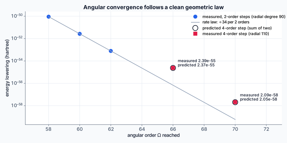A convergence model that predicts measurements it was not fitted to is the strongest evidence that the error estimate means something.

Radial degree. The energy fell by $6.1\times10^{-57}$ from degree 90 to 110. That is at $\Omega=62$, Table 2 rows 5 → 6: not strictly nested, and the figure includes any under-convergence of the degree-90 state. It then fell by $9.9\times10^{-61}$ from 110 to 118 (rows 8 → 10). If the per-order ratio were as low as 1.2, the tail beyond 118 would be about $3\times10^{-61}$; the ratio implied by the two increments, about 1.55, gives $3\times10^{-62}$. I budget the pessimistic $3\times10^{-61}$

The radial-extension cut. Extending the extra radial degree to $x<20$ instead of $x<10$ was measured at $\Omega=62$, radial degree 90: $4.2\times10^{-61}$. This is the least well-determined item, tt could be somewhat larger at radial degree 118, and a direct measurement in the final space is the obvious next check

Logarithms. $(\ln s)^3$ is worth $4.2\times10^{-62}$ but is not included in the radial-118 state; that is budgeted as-is, $(\ln s)^4$ would be orders of magnitude smaller

Solver. The last Davidson iterations change the energy by about $10^{-63}$ per iteration with slow decay, leaving a tail of about $5\times10^{-62}$.

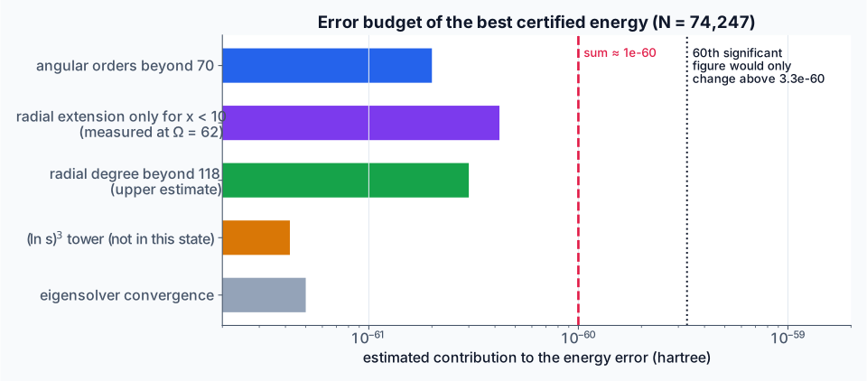The contributions sum to about 10⁻⁶⁰ hartree. The dotted line marks the error at which the 60th significant figure (59th decimal) could change.

From budget to digits. The exact energy lies about $10^{-60}$ below the bound. Decimals 51–60 of the bound read 0339042346, with 7025… after that. Lowering the energy increases the magnitude of this negative number. An error of up to $3.3\times10^{-60}$ only changes the 60th decimal (6 → at most 9); only an error beyond $3.3\times10^{-60}$ could carry into the 59th. That is more than three times the budget, and would need every estimate above to be off by a factor of three in the same direction. So

E₀ = −2.90372437703411959831115924519440444669692531111729033904234… E_h (60 significant figures, 59 decimal places)

Blue: the isotropic ladder reproduces Schwartz’s F₅₀, then flattens. Red: the anisotropic spaces with the log tower gain more than eleven further significant figures.

This is not a rigorous two-sided bound. The lower side comes from convergence analysis of measured sequences, which is the standard for record calculations but is not a theorem. A Temple- or Weinstein-type lower bound at this precision would need both a tiny residual and a certified gap to the second eigenvalue. It would be a genuinely new piece of work, and I think it is the most interesting open direction so answers on a postcard from you please.

Part V: The code, and the optimisations that made it fast

The package

Everything above runs from a small Python package, flake. It is about 1,100 lines on top of NumPy, SciPy, gmpy2 and mpmath. It has no compiled extensions, no GPU code and no multiprecision linear-algebra library. I extracted most of it from my own PhD research code base. There are six files, one per layer of the pipeline

file	lines	role
`exact.py`	125	closed-form radial moments, Gram matrices, exact inverse Cholesky, multi-double storage
`operator.py`	218	the 27-term Kronecker Hamiltonian in the white basis: build once, load anywhere
`planes.py`	192	exact digit-plane matrix products and vector algebra on float64 BLAS
`solver.py`	271	spaces as masks, the block preconditioner, Davidson, seeding, run state
`certify.py`	131	the independent exact Rayleigh quotient
`cli.py`	135	the `flake` command and the self-checks

Using it takes three commands, and a small space can run in minutes

  
pip install -e .
flake build   --order 30 --radial 30 --out f30.npz                 # exact operator, ~30 s
flake solve   --kron f30.npz --order 30 --out runs/f30 --certify    # ~5 min, N = 5,712

The record is the same three commands with bigger numbers: one build (angular order 70, radial degree 120, logs up to 3), then a chain of solve --seed runs. A script in the repository runs the whole chain.

Validation of the package itself:

flake check tests every layer in a few seconds: closed-form integrals against quadrature, exactness of the digit arithmetic (including values around $10^{15}$), and the fast Kronecker energy against the independent certifier (they agree to $3\times10^{-86}$, relative)
End to end, F10 from scratch agrees with the old, completely independent oct-double C++ code to all 41 published digits
The new certifier reproduces the production $F_{56}$ certificate to all 80 printed digits. The new solver, seeded with that state, starts exactly at its energy and residual

The optimisations

In the order they appear in the pipeline:

optimisation	what it replaces	measured effect
Kronecker factorisation in box coordinates	a dense $N\times N$ Hamiltonian	414 GB → 2.9 GB at $N = 80{,}437$; the apply becomes 52 high-precision matrix products
Exact whitening once	an oct-double factorisation per order (corrupt beyond $\Omega\approx50$)	one build serves every order and mask; the factors take minutes in gmpy2
Multi-double storage (8 float64s per exact number)	millions of Python multiprecision objects	NumPy-native files; big angular matrices go straight to integers for the GEMMs
Ozaki digit-plane GEMM	16-limb software floating point	one $\mathbf H\mathbf C$ at $F_{55}$: 516 s → 8.5 s
Skipping unused slice pairs ($s+t\le13$) before multiplying	computing all 196 slice products and discarding 91	46% fewer multiply–adds in the apply, bit-identical results
Per-row power-of-two normalisation	one scale for the whole matrix	full relative precision on rows whose magnitudes differ by $10^{18}$
Exact digit-plane vector algebra	Python-integer dot products and combinations	about half of each 70–80 s iteration removed (1.6× overall at $F_{56}$)
Cached projected matrix	recomputing $k^2/2$ dot products per iteration	one new row per iteration
Merged-sector preconditioner blocks (≤ 8,000 rows)	one block per angular order	2.5× fewer iterations; $F_{56}$ to $10^{-63}$ in 40 iterations
Regularised Cholesky $H_b-\theta+\tau\,\mathrm{diag}H_b$	`eigh` of float64 blocks	removed a stall at residual $10^{-21}$; $2.4\times10^{-55}$ in one iteration
Thick restart keeping 10 vectors (with their known $\mathbf H v$)	restarting from the Ritz vector alone	faster late convergence, no extra applies
Continuation seeds within one build	cold starts, or seeds from another build	hundreds of iterations saved per rung
Process-parallel exact builds and certification	serial gmpy2	the 26 angular matrices and 15 certifier integrals run on all cores
Cached closed-form moments	recomputing polygamma sums	every radial integral is computed once per precision

The largest single wins were structural, not low-level: the Kronecker factorisation, the whitening and the digit planes. Each changes the kind of computation rather than its speed, turning multiprecision linear algebra into ordinary BLAS. The solver-level changes then decided whether a rung converged in two hours or not at all.

Bugs that cleaning up the code flushed out

Being forced to rewrite the code for release surfaced three problems the research code had got away with. They are worth listing, because each is a generic trap

Normalising a nearly dependent vector amplifies rounding. Near convergence in a small space, a new Davidson direction can lie almost entirely inside the current subspace. After Gram–Schmidt its norm $t_n$ is tiny, and dividing by it multiplies the $2^{-280}$ orthogonality error by $1/t_n$. At F10 this cost 17 digits of normalisation ($10^{-67}$ instead of $10^{-84}$). The fix is the classic “orthogonalise, normalise, repeat while more than half the norm is lost” rule. The big production spaces never hit it
Global precision state. mpmath’s working precision is a global. The solver set it at import, the self-check lowered it to 40 digits, run in the same process, the solver’s small eigenproblem quietly lost 70 digits. The solver now sets its own precision on entry
Integer ranges in “exact” arithmetic. Described in Chapter 8: the digit format bounded every digit except the integer one, and $\mathbf H v$ on the whitened log rows is large enough to overflow it

Part VI: The numbers, and what transfers

All on a laptop

	Details
Machine	MacBook Pro, Apple M4 Pro (12 CPU cores), 24 GB unified memory
Arithmetic	float64 BLAS (Apple Accelerate) + exact integer recombination; gmpy2/MPFR for factors and certification
Exact whitening factors	minutes (radial and angular Grams at 3000 bits)
Kronecker operator build	15 min (Ω = 62), 43 min (Ω = 70); done once
One Davidson iteration at N ≈ 55,000	about 42 s
Final solves	2.7 h, 3.2 h, 3.9 h (Ω = 62, 66, 70); 3.0 h (radial 118); 3.0 h ((ln s)³)
Each certification	15 to 30 min
Peak memory	7 to 11 GB
GPU, cluster, cloud	none

Lessons from all of this

Look for a coordinate change that makes the domain a box. Once the basis is a tensor product, the operator is a short sum of Kronecker products. Memory goes from $N^2$ to a few small matrices, and every operation becomes a matrix–matrix product.
Quarantine the conditioning. It cannot be removed, only moved. Move it into the smallest objects you have (here, two Grams of at most 1,296 rows) and compute those exactly.
Error-free splitting beats software multiprecision whenever the dynamic range is bounded, as it is after whitening. Hundreds of bits at hardware BLAS speed is a 60× win. It is also preferable over DD, QD and OD datatypes which was a big learning for me.
Measure convergence per channel before adding functions. One truncation parameter hid two rates a factor of ten apart. Decoupling them bought more than all the isotropic shells after $F_{50}$.
Test the convergence model by prediction. Fit it, predict the next rung, then compute the rung.
Build an independent certifier first. Explicit trial function plus independent exact Rayleigh quotient equals a bound you can defend. It caught three serious bugs that self-checks missed.
Distrust the approximate components most, and bound the exact ones. Preconditioners and float conversions do not enter the final answer, which is exactly why their bugs survive. And “exact” arithmetic is only exact within the ranges you proved; write those ranges down and test the edges.
Use the variational principle as a bug detector. A smaller space can never beat a larger one. When it does, something is broken.
Measure slopes, not offsets. Most ideas improved the energy at fixed size. Almost none improved the rate. Only the rate reaches 60 digits.
Fit ceilings early. A decaying digits-per-function curve implies a finite ceiling, and a three-point fit tells you roughly where. Do it before investing weeks.
Continuation beats heroics. Small steps between nested spaces converge far faster than big jumps, and give you a convergence series for free.

For readers from other fields

Hopefully by now you realise that most of this has nothing to do with helium. Here is what I would take from it depending on where you come from

The Ozaki scheme deserves to be better known outside its community. Whenever a high-precision matrix product has bounded dynamic range, you can get hundreds of bits from hardware GEMMs: float64 here, but the same idea runs on integer and tensor-core units. The design question is how to make the range bounded, which is what whitening did
Kronecker structure plus masks gives you arbitrary truncation shapes at the cost of the full tensor product
Float64 assembly of a badly scaled symmetric matrix can make it indefinite. A diagonal shift of size $n\epsilon$ relative to the diagonal is the principled fix
Look for coordinates in which your basis is a tensor product, even if the domain is not obviously a box
Certify with independent code: an explicit trial function plus an exact Rayleigh quotient is a bound nobody can argue with
Measure convergence per channel. One global truncation parameter can hide rates a factor of ten apart
The anisotropic space here is a cousin of hyperbolic-cross and sparse-grid truncations. Spend degrees of freedom where the solution is rough (low angular order, high radial degree, logarithms), not uniformly
The logarithmic tower is Fock’s expansion made into basis functions. Known singular structure should be built into the basis, not approximated by brute force
“Fit the convergence law, predict the next rung, then compute it” is the same discipline as scaling-law forecasting, and just as useful for deciding where compute goes
Silent precision bugs live in the non-critical paths. A float conversion that dropped bits, an integer that overflowed and a global precision setting each changed results without raising an error
The certifier plays the role of a held-out test set: an evaluation path that shares nothing with the optimiser
Build the checker first, and keep it independent!
Refactor under bit-for-bit regression tests
Turn every invariant of your problem into an assertion. Here the variational principle (“a smaller space can never beat a larger one”) caught a bug that no unit test would have

What next

Not right now as I am helium’d out, but writing here for future reference

Measure the radial-extension cut directly in the final space, and combine radial degree 118 with the $(\ln s)^3$ tower
A rigorous lower bound (Temple/Weinstein with a certified gap) at this precision
The same machinery for helium-like ions (H$^-$, Li$^+$ and beyond), for which only the nuclear charge $Z$ in the potential weight changes (easy!)

References

E. A. Hylleraas, “Neue Berechnung der Energie des Heliums im Grundzustande, sowie des tiefsten Terms von Ortho-Helium”, Z. Phys. 54, 347 (1929).
G. Temple, “The theory of Rayleigh’s principle as applied to continuous systems”, Proc. R. Soc. Lond. A 119, 276 (1928).
E. A. Hylleraas and B. Undheim, “Numerische Berechnung der 2S-Terme von Ortho- und Par-Helium”, Z. Phys. 65, 759 (1930); J. K. L. MacDonald, “Successive approximations by the Rayleigh–Ritz variation method”, Phys. Rev. 43, 830 (1933).
V. A. Fock, “On the Schrödinger equation of the helium atom”, Izv. Akad. Nauk SSSR, Ser. Fiz. 18, 161 (1954).
T. Kato, “On the eigenfunctions of many-particle systems in quantum mechanics”, Commun. Pure Appl. Math. 10, 151 (1957).
C. L. Pekeris, “1¹S and 2³S states of helium”, Phys. Rev. 115, 1216 (1959).
K. Frankowski and C. L. Pekeris, “Logarithmic terms in the wave functions of the ground state of two-electron atoms”, Phys. Rev. 146, 46 (1966).
E. R. Davidson, “The iterative calculation of a few of the lowest eigenvalues and corresponding eigenvectors of large real-symmetric matrices”, J. Comput. Phys. 17, 87 (1975).
J. Olsen, P. Jørgensen and J. Simons, “Passing the one-billion limit in full configuration-interaction (FCI) calculations”, Chem. Phys. Lett. 169, 463 (1990).
T. Helgaker and W. Klopper, “Perspective on Hylleraas’ helium paper”, Theor. Chem. Acc. 103, 180 (2000).
G. W. F. Drake, M. M. Cassar and R. A. Nistor, “Ground-state energies for helium, H⁻, and Ps⁻”, Phys. Rev. A 65, 054501 (2002).
V. I. Korobov, “Nonrelativistic ionization energy for the helium ground state”, Phys. Rev. A 66, 024501 (2002).
C. Schwartz, “Further computations of the He atom ground state”, arXiv:math-ph/0605018 (2006).
H. Nakashima and H. Nakatsuji, “Solving the Schrödinger equation for helium atom and its isoelectronic ions with the free iterative complement interaction method”, J. Chem. Phys. 127, 224104 (2007).
K. Ozaki, T. Ogita, S. Oishi and S. M. Rump, “Error-free transformations of matrix multiplication by using fast routines of matrix multiplication and its applications”, Numer. Algorithms 59, 95 (2012).
M. Joldes, J.-M. Muller, V. Popescu and W. Tucker, “CAMPARY: Cuda Multiple Precision Arithmetic Library and Applications”, Mathematical Software – ICMS 2016, LNCS 9725 (2016).
My earlier post, “A Modern Implementation of Pekeris’ Helium Calculation”.

This post is licensed under CC BY 4.0 by the author.

weight	in \((s,t,u)\)	as box monomials \(s^{d_l}\xi^{d_x}\eta^{d_b}\)
overlap / \(\Psi_s^2,\Psi_t^2,\Psi_u^2\)	\(u(s^2-t^2)\)	\(s^3\xi - s^3\xi^3\eta^2\)
\(\Psi_s\Psi_u\) cross term	\(s(u^2-t^2)\)	\(s^3\xi^2 - s^3\xi^2\eta^2\)
\(\Psi_t\Psi_u\) cross term	\(t(s^2-u^2)\)	\(s^3\xi\eta - s^3\xi^3\eta\)
potential	\(s^2-t^2-4Zsu\)	\(s^2 - s^2\xi^2\eta^2 - 4Z\,s^2\xi\)