Try the code yourself!

Click the following button to launch an ipython notebook on Google Colab which implements the code developed in this post:

The Problem:

We want to solve the following standard eigenvalue problem

\[ \mathbf{A}\Psi = \lambda\Psi, \]

where \(\mathbf{A}\) is the lesp matrix, \(\Psi\) is the eigenvector and \(\lambda\) the eigenvalue. The lesp matrix is a tridiagonal matrix with real, sensitive eigenvalues, with a \(5 \times 5\) example seen in equation (1).

\[ \mathbf{M} = \begin{pmatrix} -5 & 2 & 0 & 0 & 0 \\
\frac{1}{2} & -7 & 3 & 0 & 0 \\
0 & \frac{1}{3} & -9 & 4 & 0 \\
0 & 0 & \frac{1}{4} & -11 & 5 \\
0 & 0 & 0 & \frac{1}{5} & -13 \\
\end{pmatrix} \tag{1} \]

We are going to numerically show that the eigenvalues of a matrix \(\mathbf{A}\) are equal to the eigenvalues of its matrix transpose, \(\mathbf{A}^T\), easily proved as follows

where \(\mathbf{I}\) is the identity matrix. If you do not want to write your own function to construct the lesp matrix then you are in luck, there is a python library, rogues, which has one built in.

The following python code calculates the eigenvalues of \(\mathbf{A}\) and \(\mathbf{A}^T\) and displays them using seaborn.

1
2
3
4
5
6
7
8
9
10
11
12
13
14
15
16
17
18
19
20
21
22
23
24
25
26
27
28
29
30
31
32
33
34

from rogues import lesp
from matplotlib import pyplot
import seaborn as sns 
from scipy.linalg import eigvals

sns.set()
palette = sns.color_palette("bright")

# Dimension of matrix
dim = 100
# get lesp matrix
A = lesp(dim)
# Transpose matrix A
AT = A.T
# Calculate eigenvalues of A
Aev = eigvals(A)
# Calculate eigenvalues of A^T
ATev = eigvals(A.T)
# Extract real and imaginary parts of A
A_X = [x.real for x in Aev]
A_Y = [x.imag for x in Aev]
# Extract real and imaginary parts of A^T
AT_X = [x.real for x in ATev]
AT_Y = [x.imag for x in ATev]

# Plot
ax = sns.scatterplot(x=A_X, y=A_Y, color = 'gray', marker='o', label=r'$\mathbf{A}$')
ax = sns.scatterplot(x=AT_X, y=AT_Y, color = 'blue', marker='x', label=r'$\mathbf{A}^T$')
# Give axis labels
ax.set(xlabel=r'real', ylabel=r'imag')
# Draw legend
ax.legend()

pyplot.show()

This produces the following plot of the eigenvalues for a \(100 \times 100 \) matrix.

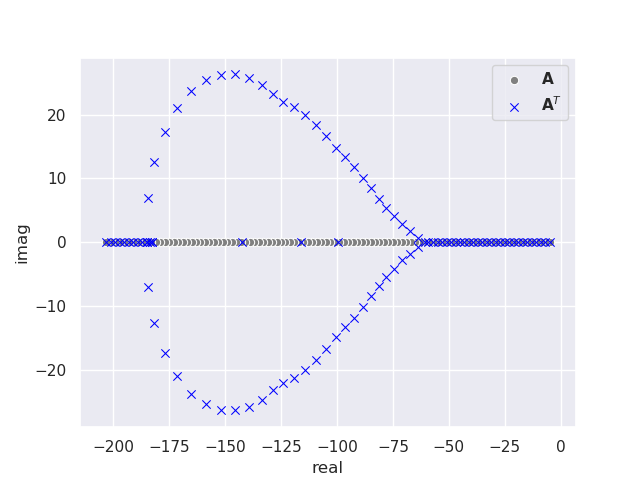
Something is wrong, most of the eigenvalues of matrix \(\mathbf{A}\) are not equal to the eigenvalues of \(\mathbf{A}^T\), even though they should be identical. Some of them also have complex components! There is no error with the program; this discrepancy is caused by a loss of numerical accuracy in the eigenvalue calculation due to the limitation of hardware double precision (16-digit).

The Solution:

The scipy eigvals function calls LAPACK routine _DGEEV which first reduces the input matrix to upper Hessenberg form by means of orthogonal similarity transformations. The QR algorithm is then used to further reduce the matrix to upper quasi-triangular Schur form, \(\mathbf{T}\), with 1 by 1 and 2 by 2 blocks on the main diagonal. The eigenvalues are computed from \(\mathbf{T}\).

For most applications this will produce very accurate eigenvalues, but when a problem is ill-conditioned, or a small change to the input matrix results in a significant change to the eigenvalues; more numerically stable methods are required. Failing this, higher working precision is required such as quadruple (32-digit), octuple (64-digit) or even arbitrary precision. If you are losing precision in a calculation it is always advised to first analyse the methods and algorithms you are using to see if they can be improved. Only after doing this is it desirable to increase the working precision. Extended precision calculations take significantly longer than double precision calculations as they are run in software rather than on hardware.

Increasing precision is simple in python with the use of the mpmath library. Note that this library is incredibly slow for large matrices, so is best avoided for most applications. The following code calculates the same eigenvalues as before, this time at quadruple, 32-digit precision.

1
2
3
4
5
6
7
8
9
10
11
12
13
14
15
16
17
18
19
20
21
22
23
24
25
26
27
28
29
30
31
32
33
34
35
36
37

from rogues import lesp
from matplotlib import pyplot
import seaborn as sns 
from scipy.linalg import eigvals
from mpmath import *
# Set precision to 32-digit
mp.dps = 32

sns.set()
palette = sns.color_palette("bright")

# Dimension of matrix
dim = 100
# Lesp matrix
A = lesp(dim)
# Transpose matrix A
AT = A.T
# Calculate eigenvalues of A
Aev, Eeg = mp.eig(mp.matrix(A))
# Calculate eigenvalues of A^T
ATev, ETeg = mp.eig(mp.matrix(AT))
# Extract real and imaginary parts of A
A_X = [x.real for x in Aev]
A_Y = [x.imag for x in Aev]
# Extract real and imaginary parts of A^T
AT_X = [x.real for x in ATev]
AT_Y = [x.imag for x in ATev]

# Plot
ax = sns.scatterplot(x=A_X, y=A_Y, color = 'gray', marker='o', label=r'$\mathbf{A}$')
ax = sns.scatterplot(x=AT_X, y=AT_Y, color = 'blue', marker='x', label=r'$\mathbf{A}^T$')
# Give axis labels
ax.set(xlabel=r'real', ylabel=r'imag')
# Draw legend
ax.legend()

pyplot.show()

This produces the following plot of the eigenvalues for a \(100 \times 100 \) matrix.

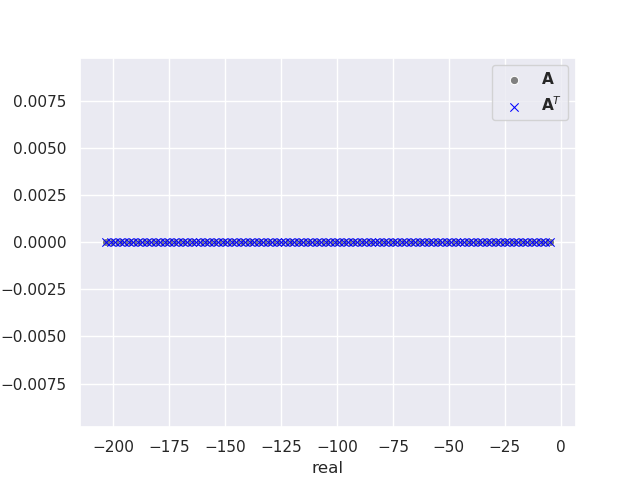
Success! We have shown that the eigenvalues of \(\mathbf{A}\) are equal to the eigenvalues of \(\mathbf{A}^T\), equation (1) and all eigenvalues are real. This particular example highlights a recurring theme within computational studies of quantum systems. Quantum simulations of atoms and molecules regularly involve ill-conditioned standard and generalized eigenvalue problems. Numerically stable algorithms exist for such problems, but these occasionally fail leaving us to brute force the calculation with higher precision to minimize floating point rounding errors.

The next post will discuss better ways to implement higher precision in numerical calculations.