Try the code yourself!

Click the following button to launch an ipython notebook on Google Colab which implements the code developed in this post:

The Problem:

We want to solve the Schrödinger equation for the hydrogen atom

\[ \hat{H}\psi = E\psi. \tag{1} \]

Where \(\hat{H} \) is the Hamiltonian, \(\psi\) the wavefunction and \(E\) the energy. This is the textbook system studied in quantum mechanics as it is the most simple consisting of just a single proton and electron. The hydrogen atom is exactly solvable using a series solution method built on associated Laguerre polynomials, but this is T>T so we are going to solve it numerically using a very powerful technique, the variational method.

Variational Method

Consider the wave equation given in equation (1). If we multiply both sides by \(\psi\) and integrate over all space we end up with the following

\[ E = \frac{\int \psi \hat{H}\psi \text{d}\tau}{\int \psi^2 \text{d}\tau}. \tag{2} \]

When \(\psi\) is complex this becomes

\[ E = \frac{\int \psi^* \hat{H} \psi \text{d}\tau}{\int \psi^* \psi \text{d}\tau}. \tag{3} \]

We can now calculate the energy, \(E\) if we know the wavefunction, \(\psi\). The first step is to guess the wavefunction using some physical intuition as to how it might behave given certain criteria. If you are concerned with the concept of guessing in science then have a listen to Richard Feynman on the scientific process.

It is unlikely that our guess will be the exact wavefunction, but by labelling it as \(\psi_1\) it will give us a value of the energy, \(E_1\). We can now guess a second wavefunction, \(\psi_2\) resulting in an energy value \(E_2\) and if desired we could guess even more wavefunctions, there is no limit. The variational principle tells us that if \(E_g\) is the exact ground state energy then both \(E_1\) and \(E_2\) will always be greater than \(E_g\) unless we somehow guessed the exact wavefunction. We can represent the variational principle via the following inequality

\[ \frac{\int\psi^* \hat{H} \psi \text{d}\tau}{\int \psi^* \psi \text{d}\tau} \ge E_g. \tag{4} \]

If we choose the lowest of the \(E_n\)’s we calculate from our choice of functions \(\psi_n\), which we will call \(E_i\), this must satisfy the following:

1) \(E_i\) will be the closest to the true energy, \(E_g\),

2) \(E_i\) will always be greater than \(E_g\),

3) \(\psi_i\) will be the closest approximation to the true wavefunction \(\psi_g\).

When choosing our basis to build the wavefunction, we can introduce variational parameters which can be varied during the calculation, increasing the flexibility of our chosen wavefunction. The more variational parameters introduced the greater the wavefunction flexibility and thus the better “fit” to the true wavefunction. This comes with a greater computational cost, hence compromise is needed between desired accuracy and the number of variational parameters.

Variational Method for the Hydrogen Atom

The Hamiltonian for the hydrogen atom is as follows

\[ \hat{H} = -\frac{\hbar^2}{2\mu}\nabla^2 - \frac{e^2}{r}, \tag{5} \]

where \(\mu\) represents the reduced mass of the proton-electron pair (\(\mu \approx 1\) for the hydrogen atom) and \(r\) the inter-particle separation. We can now decide an educated guess for our wavefunction form, first thinking about what happens when the electron is far away from the proton. In this instance we would expect \(\psi \rightarrow 0\) asymptotically due to the electron being bound to the proton, hence the probability of it being an infinite distance away from the proton will tend to 0. A sensible wavefunction ansatz could be a negative exponential function of the form

\[ \psi_1 = e^{-c r}, \tag{6} \]

where \(c\) is a single variational parameter. Our Hamiltonian from equation (5) must act on the wavefunction which we can now do by forming the time independent Shrödinger equation seen in equation (1). We need to give our Laplacian operator in the Hamiltonian the correct form; and this is where the maths becomes a little trickier, but really there is just a lot of little, easy steps involved. Due to the spherical symmetry, it is best to represent the Laplacian using spherical polar coordinates

\[ \nabla^2 = \frac{\partial^2}{\partial r^2} + \frac{2}{r}\frac{\partial}{\partial r} + \frac{1}{r^2}\left(\frac{\partial^2}{\partial \theta^2} + \frac{1}{\text{tan}\theta}\frac{\partial}{\partial \theta} + \frac{1}{\text{sin}^2\theta}\frac{\partial^2}{\partial \phi^2}\right) \tag{7} \]

We can simplify this by recognising that our wavefunction does not contain any angular components as we are concerned with the ground state of the hydrogen atom which is spherically symmetric, only requiring the radial solution. The Laplacian can now be written as

\[ \begin{aligned} \nabla^2 & = \frac{\partial^2}{\partial r^2} + \frac{2}{r}\frac{\partial}{\partial r} \\
\nabla^2\psi_1 & = \left(c^2 - \frac{2c}{r}\right)e^{-cr} \end{aligned} \tag{8} \]

We can now construct an energy expression using equation (4) and equation (8)

\[ \begin{aligned} E(c) \equiv \frac{\int \psi_1\hat{H}\psi_1\text{d}\tau}{\int \psi_1\psi_1\text{d}\tau} & = \frac{\frac{(c\hbar^2 -2e^2)\pi}{2c^2}}{\frac{\pi}{c^3}} \\
& = \frac{\hbar^2c^2}{2} - e^2c \end{aligned} \tag{9} \]

By recasting the problem into atomic units we can dispose of the annoying \(\hbar\) and \(e\) giving.

\[ E(c) = \frac{c^2}{2} - c. \]

A plot of \(E(c)\) is seen below

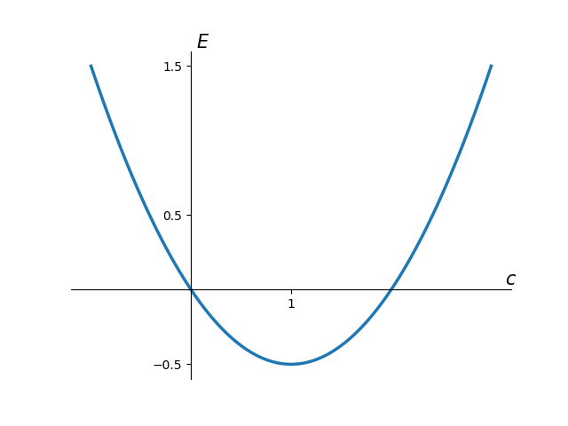
It is clear where the minimum is from a visual inspection, but we want the computer to tell us; as for more complex examples it is impossible to visualise the function due to it existing in \(n\)-dimensions. The following python snippet takes our function and varies the parameter \(c\) to obtain the lowest value of the ground state energy. This uses the minimize function of the scipy optimize library containing a vast array of options for non linear parameter optimisation; a subject of a future T>T post.

1
2
3
4
5
6
7
8
9
10
11
12
13
14

from scipy.optimize import minimize

def min(c):
    # Define our energy function
    E = (c**2/2) - c
    # print off useful information each optimisation cycle
    print("c = {:.6f}, Energy = {:.16f}".format(c[0], E[0]))
    
    return E

# Provide an initial guess for the variational parameter c
c = 5
# Optimise the min function by varying c with a tolerance of 1e-6
hydrogen_gs = minimize(min, c, tol=1e-6) 

The output of this program is the following:

1
2
3
4
5
6
7
8
9
10
11
12

c = 5.000000, Energy = 7.5000000000000000
c = 5.000000, Energy = 7.5000000596046448
c = 5.000000, Energy = 7.5000000000000000
c = 3.990000, Energy = 3.9700500000000005
c = 3.990000, Energy = 3.9700500000000005
c = 3.990000, Energy = 3.9700500445544726
c = 1.605218, Energy = -0.3168557476139684
c = 1.605218, Energy = -0.3168557476139684
c = 1.605218, Energy = -0.3168557385955213
c = 1.000000, Energy = -0.5000000000000000
c = 1.000000, Energy = -0.5000000000000000
c = 1.000000, Energy = -0.5000000000000000

Success! The final result from our minimisation program is

\[ E = -0.5\ \text{hartrees}, \]

when \(c = Z = 1\) where \(Z\) represents the nuclear charge which for hydrogen is 1. This is the location of the minimum in the above plot of the energy expression; and also the true ground state energy of the hydrogen atom in atomic units. We luckily (or perhaps this was a setup…) selected the exact wavefunction ansatz. Our optimised wavefunction is thus

\[ \psi_1 = e^{-1r}, \tag{10} \]

or more generally

\[ \psi_1 = e^{-Zr}, \tag{11} \]

We chose our wavefunction ansatz wisely, but what if we mistakenly selected a different functional form? Consider a Gaussian function

\[ \psi_2 = e^{-cr^2}, \]

where the difference from equation (6) is the power of 2 in the exponent of \(r\). Following the same process as above with this new wavefunction form gives the following energy expression

\[ E(c) = \frac{3\hbar^2}{2}c - \frac{4e^2\sqrt{2}}{\sqrt{\pi}}c^{\frac{1}{2}}. \]

This energy function using our Gaussian ansatz, \(\psi_2\) has been plotted along with the one above calculated using \(\psi_1\),

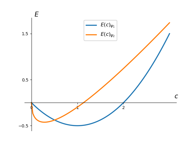
This new energy function is noticeably different than the original one. If we minimise this function with respect to \(c\) we get

\[ E = -0.424413 \ \text{hartrees}, \] when \(c = 0.282933\). This is further away from the true value of \(E = -0.5\ \text{hartrees}\) than our first guess. This highlights the importance of selecting a suitable basis for your wavefunction. Travelling further down the rabbit hole of quantum mechanics, you quickly find that Gaussian functions are actually a favoured basis set for wavefunctions; due to a multitude of useful mathematical properties even though they fail to satisfy certain physical properties. In this post we only used a single function for our wavefunction but in reality you can form a linear combination of functions with a multitude of variational parameters to aid in convergence of the energy.

Conclusions

We used the variational method and a selected wavefunction form to construct an energy expression in terms of a variational parameter \(c\). We minimised this function to find the ground state energy of the hydrogen atom, which by luck matched the exact ground state energy. We then used a Gaussian function as our wavefunction ansatz and found that it produced an energy higher than our first wavefunction; highlighting the importance of the initial wavefunction guess to calculate the lowest energy. Future T>T posts will explore this vast research area in more detail.