T>T: Hartree Fock Theory in 100 Lines
This post is part of a series on Hartree-Fock theory:
- Restricted Hartree-Fock in 100 Lines: You are here
- Unrestricted Hartree-Fock in 100 Lines: This lifts the closed-shell restriction, adds spin degrees of freedom
- The Integrals at the Heart of Hartree-Fock Theory: Derives every integral used in this post from scratch, with interactive visualisers. This is useful when you get to the integral pasrt of this post.
Try the code yourself!
Click the following button to launch an ipython notebook on Google Colab which implements the code developed in this post:
![]()
In a previous post we looked at the hydrogen atom which is an exactly solvable two-particle quantum system. If we consider a system with a nucleus and two-electrons, a three-particle system, such as the helium atom, the quantum mechanical equations can no longer be solved exactly. This poses a towering hurdle to overcome as looking at the periodic table shows that every chemical element other than hydrogen contains more than 1 electron; some of them containing hundreds of electrons. If the equations of quantum mechanics cannot exactly solve any system with more than one electron then do we just throw in the towel and go solve something else? No…
We need to relax the demand for an exact solution, and instead settle for an approximate solution. Quantum physics and chemistry has been developing methods to calculate these approximate solutions for almost a century, and there are now a wide variety of sophisticated methods. If we trace back their origins we arrive at a method called Hartree Fock theory or HF for short. Hartree Fock theory provides a means of approximating the wave function and energy of a many-electron system in it’s ground state. The theory was developed in the late 1920’s but still underpins most modern many-electron electronic structure methods.
The aim of this post is to bridge the gap between Hartree Fock theory discussed in a textbook and how it is actually programmed. No published work I have seen accomplishes this and as Hartree Fock is the OG many-electron theory, it deserves a thorough guide and an appreciation of its intricacies. To start, we will discuss the theory in very simple terms before going more indepth and developing our own Hartree Fock program using just 100 lines of python code. We could make it shorter but the aim is to not compromise the readability of the code.
Restricted Hartree Fock Theory Made Simple
Consider the helium atom depicted below, consisting of a central nucleus, surrounded by two electrons.
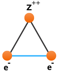
The reason the equations of quantum mechanics are not solvable exactly for this system is due to the interaction between the two electrons highlighted in blue which we term electron correlation. In the hydrogen atom this interaction is abscent, hence can be solved exactly. If we cannot solve helium exactly then how can we approximate it? If we look at the greatly simplified helium schematic it almost looks like two hydrogen atoms stacked on top of each other. This simple observation is at the core of Hartree Fock theory, as it is built upon one-electron operators. We take something we know, the hydrogen atom, and use them as building blocks to construct more complex atoms and molecules.
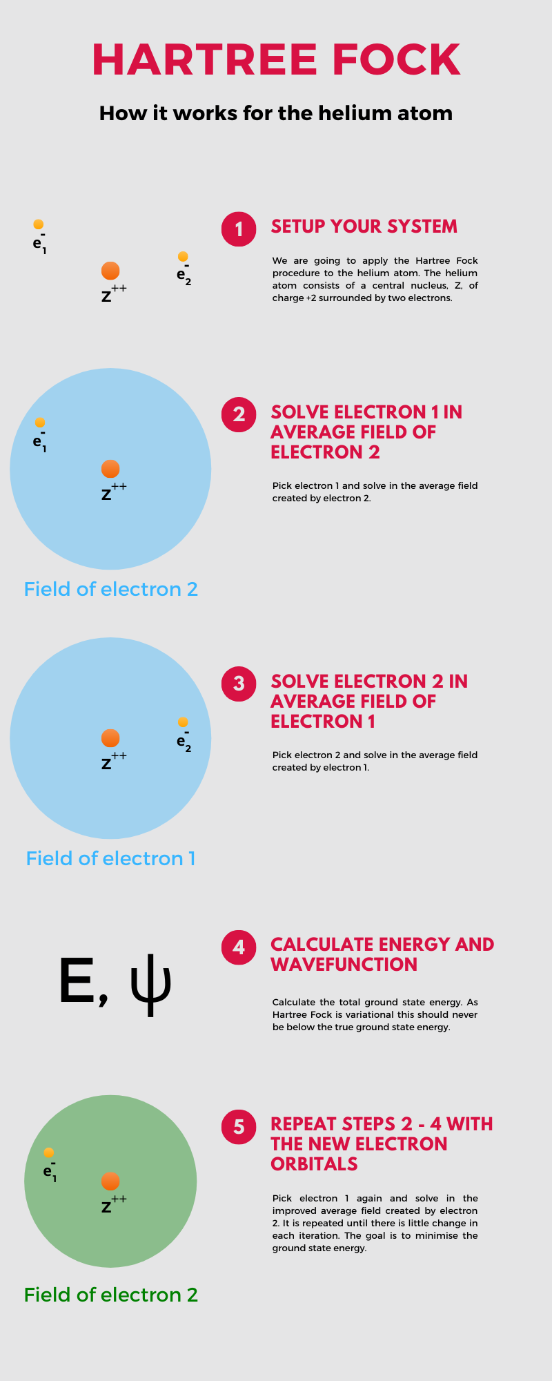
The tricky part is how to introduce the interaction between the electrons, the electron correlation. Each electron repels the other electron so that their motion is dependent on the motion of the other one. This non-separability of the electron orbits introduces the complexity into the problem, but it also suggests a possible way out. Consider one electron and disregard its instantaneous interaction with the other electron, instead imagining it to move in an average field created by the other electron. We solve the associated quantum mechanical equations and are left with a new orbital. We now switch to the other electron and repeat the process this time using the new orbital expression as our average field. We repeat this process until the results do not change. I created the following infographic to explain this procedure more clearly.
Restricted Hartree Fock Theory in Detail
It is now time to develop our own Hartree Fock program. This section requires a firm knowledge in quantum mechanics and mathematics, so be prepared. From the infographic above we discuss “solving” quantum mechanical equations but it helps to know what we are actually solving; the electronic Schrödinger equation. This results from the time-independent Schrödinger equation after invoking the Born-Oppenheimer approximation
\[ \hat{H}\psi = E\psi, \tag{1} \]
where the Hamiltonian operator for the helium atom has the form
\[ \hat{H} = -\frac{1}{2}\nabla_1^2 - \frac{1}{2}\nabla_2^2 + \frac{Z}{r_1} + \frac{Z}{r_2} + {\frac{1}{r_{12}}}, \tag{2} \]
with the Born-Oppenheimer approximation invoked by removing the mass polarisation term. Let us now assume that our wavefunction is just a product of one-electron wavefunctions
\[ \psi(\mathbf{r}_1, \mathbf{r}_2) = \phi_1(\mathbf{r}_1)\phi_2(\mathbf{r}_2). \tag{3} \]
This is referred to as the Hartree product which is a sensible starting point, but this wavefunction fails to satisfy one of the most fundamental laws of quantum mechanics, the antisymmetry principle. This states that a wavefunction describing fermions should be antisymmetric (i.e. changes sign) with respect to the interchange of any set of space-spin coordinates. Textbooks tend to denote space-spin coordinates as \(\mathbf{x} = \lbrace\mathbf{r}, \omega\rbrace\) where \(\mathbf{r}\) represents the spatial degrees of freedom and \(\omega\) the spin coordinate. In most Hartree Fock applications the spin is integrated off early on in the process as it can make things annoyingly complicated later on. Introducing these space-spin coordinates into our Hartree product gives
\[ \psi(\mathbf{x}_1, \mathbf{x}_2) = \chi_1(\mathbf{x}_1)\chi_2(\mathbf{x}_2), \tag{4} \]
where we have also substituted spin orbitals, \(\chi(\mathbf{x})\) in place of the spatial orbitals \(\phi(\mathbf{r})\). This still fails to satisfy the antisymmetry principle which we now demonstrate. Consider switching the position of the two electrons, \(1 \leftrightarrow 2\)
\[ \psi(\mathbf{x}_2, \mathbf{x}_1) = \chi_1(\mathbf{x}_2)\chi_2(\mathbf{x}_1). \tag{5} \]
The sign of the wavefunction has not changed, thus it is an incorrect wavefunction. We now introduce the Fock into our Hartree Fock method with the use of Slater determinants. A Slater determinant is a determinant of spin orbitals which represents an antisymmetrised wavefunction. For the helium atom this looks like
\[ \psi(\mathbf{x}_1, \mathbf{x}_2) = \frac{1}{\sqrt{2!}} \begin{vmatrix} \chi_1(\mathbf{x}_1) & \chi_2(\mathbf{x}_1) \\
\chi_1(\mathbf{x}_2) & \chi_2(\mathbf{x}_2) \end{vmatrix}. \tag{6} \]
By expanding this determinant we get the following wavefunction form
\[ \psi(\mathbf{x}_1, \mathbf{x}_2) = \frac{1}{\sqrt{2}} \left[\chi_1(\mathbf{x}_1)\chi_2(\mathbf{x}_2) - \chi_2(\mathbf{x}_1)\chi_1(\mathbf{x}_2) \right], \tag{7} \]
which is just a linear combination of the possibilities and does obey the antisymmetry principle. Another consequence of forming the Slater determinant is that if any two rows or columns are identical then the determinant is zero. This shows that the wavefunction dissapears if two electrons have the same quantum numbers, required by the Pauli exclusion principle which is a consequence of the antisymmetry principle.
Hartree Fock Equation
As discussed earlier, Hartree Fock theory is built upon one-electron operators with each electron considered to move in the electrostatic field of the nuclei and the average field of the \(N-1\) electrons. One of these one electron operators acts on an orbital to produce an orbital energy and associated orbital wavefunction. The following represents the Hartree Fock equation for a spin orbital, \(\chi_i\), occupied by electron 1
\[ f(\mathbf{x_1})\chi_i(\mathbf{x_1}) = \epsilon_i\chi_i(\mathbf{x_1}). \tag{8} \]
with \(f(\mathbf{x_1})\) representing the one-electron Fock operator and \(\epsilon_i\) the one-electron orbital energy. By integrating out the spin, we are left with the closed-shell spatial Hartree Fock equation
\[ f(\mathbf{r_1})\psi_i(\mathbf{r_1}) = \epsilon_j\psi_i(\mathbf{r_1}). \tag{9} \]
Note, the energy of the spin orbital, \({\epsilon_i}\) is equal to the energy of the spatial orbital, \(\epsilon_j\). This equation is just a simple eigenvalue equation, where the Fock operator, \(f(\mathbf{r_1})\) acts on the spatial function, \(\psi_i(\mathbf{r_1})\) to produce eigenvalues, \(\epsilon_j\). This highlights that the Fock operator is an effective one-electron operator, as it acts on a one-electron function. The Fock operator has the form
\[ f(\mathbf{r_1}) = h(\mathbf{r_1}) + \sum_{a}^{N/2}\int \psi_a^*(\mathbf{r_2})(2-P_{12})r_{12}^{-1}\psi_a(\mathbf{r_2})\text{d}\mathbf{r_2}, \tag{10} \]
where \(P_{12}\) represents the parity operator. A more convenient and recognisable form is
\[ f(1) = h(1) + \sum_{a}^{N/2}2J_a(1) - K_a(1), \tag{11} \]
The Fock operator contains all the relevant interactions between particles, with terms defined as follows:
- \(f(1)\): Fock operator
- \(h(1)\): Nucleus-electron kinetic energy and potential attraction to all nuclei
- \(J_a(1)\): Coulomb operator -> Electron-electron repulsion
- \(K_a(1)\): Exchange operator -> Electron-electron exchange
There are two electrons in each orbital forming \(N\) total electrons. The sum is over the \(N/2\) occupied orbitals, \(\psi_a\). The closed-shell Coulomb operator, \(J\) and exchange operator, \(K\) have the following forms
\[ J_a(1) = \int \psi_a^*(2)r_{12}^{-1}\psi_a(2)\text{d}\mathbf{r_2}, \tag{12} \]
\[ K_a(1)\psi_i(1) =\left[\int \psi_a^*(2)r_{12}^{-1}\psi_i(2)\text{d}\mathbf{r_2}\right]\psi_a(1). \tag{13} \]
The exchange operator is a purely quantum mechanical entity with no classical analogue, hence must act on a wavefunction. In its current state, this mathematics will be cumbersome to program on a computer; so lets write it in a form that it can better understand, using the language of matrices.
Roothaan-Hall Equations
This is where Restricted Hartree Fock begins from a computational standpoint. Equation (9) represents a complicated integro-differential equation, meaning it involves both integrals and derivatives of a function. Roothaan and Hall independently showed that by introducing a set of known spatial basis functions, the differential equation could be converted to a set of algebraic equations. This meant that standard matrix techniques could be used to achieve a solution.
This is more like it! Computers and matrices were made for each other, and the complicated integro-differential equation transforms into a much simpler matrix equation
\[ \mathbf{F}\mathbf{C} = \mathbf{S}\mathbf{C}\boldsymbol{\epsilon}, \tag{14} \]
where \(\mathbf{F}\) represents the Fock matrix, \(\mathbf{C}\) is a \(K \times K\) square matrix of the expansion coefficients, \(\mathbf{S}\) is the overlap matrix and \(\boldsymbol{\epsilon}\) is a diagonal matrix of the orbital energies, \(\epsilon_i\). The overlap matrix, \(\mathbf{S}\) is required as basis sets are not usually orthonormal sets. The basis functions tend to be normalised, but they are not always orthogonal to each other. In order to write the Roothaan-Hall equations in the form of a matrix eigenvalue problem, the basis needs to be orthogonalised; so for basis functions that are not orthogonal, we include the \(\mathbf{S}\) matrix in order to ensure the orthonormality. The overlap matrix elements have the following form
\[ S_{\mu \nu} = \int \phi_\mu^*(\mathbf{r})\phi_\nu(\mathbf{r})\text{d}\mathbf{r}. \tag{15} \]
The Roothan-Hall equations cannot be solved directly because the Fock matrix depends on the Coulomb and exchange integrals which depend on the spatial wavefunction meaning there is an inter-dependency issue. We thus follow a Self Consistent Field (SCF) procedure where new coefficients \(C_{ij}\) are obtained each iteration, continuing until the convergence criteria has been met. We now introduce the charge density matrix which we will use to calculate the Fock matrix, \(\mathbf{F}\).
Charge Density Matrix
A charge density matrix is a probability distribution function of an electron, described by a spatial function, \(\psi_a(r)\). The probability of finding this electron in a volume element \(\text{d}\mathbf{r}\) at a point \(\mathbf{r}\) is simply \(\lvert\psi_a(r)\rvert^2 \text{d}\mathbf{r}\), which in turn means the probability distribution function is \(\lvert\psi_a(r)\rvert^2\).
For the Closed-shell Hartree Fock problem, described by a single determinant wave function with all orbitals doubly occupied, the total charge density is given by
\[ \rho(\mathbf{r}) = 2\sum\limits_{a}^{N/2}|\psi_a(\mathbf{r})|^2. \tag{16} \]
The probability of finding any electron in the volume element, \(\text{d}\mathbf{r}\) at \(\mathbf{r}\) is \(\rho (r) \text{d}\mathbf{r}\). We can also calculate the total number of electrons by integrating the charge density
\[ \int \rho (\mathbf{r})\text{d}\mathbf{r} = 2\sum\limits_{a}^{N/2}\int|\psi_a(\mathbf{r})|^2 \text{d}\mathbf{r} = 2\sum\limits_{a}^{N/2}1 = N, \tag{17} \]
assuming \(\psi_a(\mathbf{r})\) normalises to one. For a single determinant, the total charge density is just the sum of the charge densities for each of the electrons.
Now insert a generic orbital expression, \(\psi_a(\mathbf{r}) = \sum C\phi(\mathbf{r})\) into equation (16). The function, \(\phi(\mathbf{r})\) represents the basis function you want, e.g. exponential function, Hermite polynomial etc… and \(C\) represents the weighting coefficient of that particular function, i.e. how much it contributes to the total wavefunction, \(\psi_a(\mathbf{r})\).
\[ \begin{aligned} \rho(\mathbf{r}) & = 2\sum\limits_{a}^{N/2}\psi_{a}^* (\mathbf{r})\psi_a(\mathbf{r}) \\
& = 2 \sum\limits_{a}^{N/2}\sum\limits_{\nu}C_{\nu a}^* \phi_{\nu} ^* (\mathbf{r})\sum\limits_{\mu}C_{\mu a}\phi_\mu(\mathbf{r}) \\
& = \sum\limits_{\mu \nu}P_{\mu\nu}\phi_{\mu}(\mathbf{r})\phi_{\nu} ^*(\mathbf{r}) \end{aligned} \tag{18} \]
where \(P_{\mu\nu}\) represents the matrix elements of the charge density matrix, \(\mathbf{P}\)
\[ P_{\mu\nu} = 2\sum\limits_{a}^{N/2} C_{\mu a}C_{\nu a}^*. \tag{19} \]
The charge density matrix is built using the coefficients of the basis set, and given a set of basis functions, \({\phi_\mu }\), the matrix \(\mathbf{P}\) specifies the charge density, \(\rho(\mathbf{r})\) of the electrons in your system. If we look back at our Fock matrix expression, equation (11), and introduce this basis \({\phi_\mu}\), we get
\[ \begin{aligned} F_{\mu\nu} & = \int \phi_{\mu}^* (1)f(1)\phi_\nu(1)\text{d}\mathbf{r_{1}} \\
& =\int \phi_{\mu}^* (1)h(1)\phi_{\nu}(1)\text{d}\mathbf{r_{1}} + \sum\limits_{a}^{N/2}\int\phi_{\mu}^* (1)[2J_a (1) - K_a (1)]\phi_{\nu}(1)\text{d}\mathbf{r_{1}} \\
& =H_{\mu\nu}^\text{core} + \sum\limits_{a}^{N/2} 2(\mu\nu\lvert aa) - (\mu a\lvert a\nu) \end{aligned} \tag{20} \]
where \((\mu\nu\lvert aa)\) is shorthand notation for a two-electron integral. Our choice of wavefunction will involve some form of linear expansion given by
\[ \psi_i = \sum\limits_{\mu=1}^{K} C_{\mu i}\phi_\mu, \hspace{1cm} i =1,2,\ldots,K. \tag{21} \]
We now insert this expansion into the two-electron terms giving us our final expression for the Fock matrix
\[ \begin{aligned} F_{\mu\nu} & = H_{\mu\nu}^\text{core} + \sum\limits_{a}^{N/2}\sum\limits_{\lambda\sigma}C_{\lambda a}C_{\sigma a}^* [2(\mu\nu|\sigma\lambda) - (\mu\lambda|\sigma\nu)] \\
& = H_{\mu\nu}^\text{core} + \sum\limits_{\lambda\sigma} P_{\lambda\sigma}[(\mu\nu|\sigma\lambda) - \frac{1}{2}(\mu\lambda|\sigma\nu)] \\
& = H_{\mu\nu}^\text{core} + G_{\mu\nu}, \end{aligned} \tag{22} \]
where \(G_{\mu\nu}\) is the two-electron part of the Fock matrix.
This all seems very complicated but we have now discussed all the elements we need, so lets start our program and learn on the job. We start with an overview of the Hartree Fock procedure our program should follow.
The Hartree Fock Procedure
The Hartree Fock process is as follows:
Specify system and basis set
Calculate one and two-electron integrals
Diagonalise the overlap matrix, \(\mathbf{S}\) to obtain a transformation matrix, \(\mathbf{X} \equiv \mathbf{S} ^{−1/2}\)
Provide initial guess as to the density matrix, \(\mathbf{P}\).
Calculate \(\mathbf{G}\) matrix (\(\mathbf{G} = 2\mathbf{J} - \mathbf{K}\)) using \(\mathbf{P}\) and the two-electron integrals
Obtain Fock matrix from sum of the core Hamiltonian matrix and \(\mathbf{G}\) matrix, \(\mathbf{F} = \mathbf{H}^\text{core} + \mathbf{G}\)
Calculate transformed Fock matrix, \(\mathbf{F}’ = \mathbf{X}^\dagger \mathbf{F}\mathbf{X}\)
Diagonalise \(\mathbf{F}’\) to obtain \(\mathbf{C}’\)
Calculate the coefficient matrix using, \(\mathbf{C} = \mathbf{X} \mathbf{C}’\)
These coefficients form the new density matrix, \(\mathbf{P}\)
Determine convergence of the density matrix, by comparing the new density matrix with the old density matrix within a specified criterion. If the convergence has not been met then return to step (5) with the new density matrix \(\mathbf{P}\) to form a new Fock matrix and repeat
If convergence has been met then end the SCF cycle and return desired quantities, e.g. Energy, coefficient matrix.
This process looks more difficult than it actually is. Hartree Fock theory is a wavefunction based method, meaning a wavefunction form needs to first be selected and the associated one and two-electron integrals calculated. A nice example of restricted Hartree Fock theory is given in Lewars\(^{[2]}\) for protonated helium, H-He\(^+\). This system will be borrowed as it represents some benchmark data for our own program to replicate.
1) Specify system and basis set
The basis set for this example will be the STO-1G basis set, meaning Slater-Type Orbitals-1 Gaussian, i.e. approximating a slater-type 1s orbital with a Gaussian function. The STO-1G approximations used for the hydrogen and helium 1s orbitals in a molecular environment are
\[ \begin{aligned} \phi(\text{H}) &= \phi_1 = 0.3696 \text{exp}(-0.4166|\mathbf{r} - \mathbf{R_1}|^2), \\
\phi(\text{He}) &= \phi_2 = 0.5881 \text{exp}(-0.7739|\mathbf{r} - \mathbf{R_2}|^2), \end{aligned} \]
where \(\lvert\mathbf{r} − \mathbf{R_i} \rvert\) is the distance of the electron in \(\phi_ 1\) from nucleus, \(i\) on which \(\phi_i\) is centred. The multiplicity of this singlet ground state (number of unpaired electron spins) is
\[ \text{Multiplicity = 2s + 1,} \]
where \(s\) is the total number of unpaired electron spins; so for the singlet ground state with paired electron spins, Multiplicity = 1.
2) Calculate One and Two-Electron Integrals
Calculation of one and two-electron integrals are dependent on the wavefunction form so their calculation is specific to the selected basis; and there is not a completely generic calculation route.
One-Electron Integrals
One-electron integrals make up the core Hamiltonian matrix. This contains the interaction between the nucleus and each electron in the absence of electron-electron interaction.
Kinetic Energy:
\[ T_{rs}(1) = \int\phi_r\left(-\frac{1}{2}\nabla_1^2\right)\phi_s\text{d}\nu. \tag{23} \]
Potential Energy Integral for hydrogen atom, H:
\[ V_{rs}(\text{H},1) = \int\phi_{r}\left(\frac{Z_\text{H}}{r_{\text{H} 1}}\right)\phi_s\text{d}\nu. \tag{24} \]
Potential Energy Integral for helium atom, He:
\[ V_{rs}(\text{He},1) = \int\phi_r\left(\frac{Z_\text{He}}{r_{\text{He}1}}\right)\phi_s\text{d}\nu. \tag{25} \]
where \(r_{\text{H}1}\) represents the distance of an electron from the hydrogen nucleus and \(r_{\text{He}1}\) represents the distance of an electron from the helium nucleus. Substitute the hydrogen and helium orbitals into these expressions to calculate the one-electron integrals. This can be done using Mathematica, Maple etc…
\[ \begin{aligned} T_{11} &= 0.6429 \\
T_{12} &= T_{21} = 0.2395 \\
T_{22} &= 1.1609\\
V_{11}(\text{H}) &= -1.0300\\
V_{12}(\text{H}) &= V_{21}(\text{H}) = -0.4445\\
V_{22}(\text{H}) &= 1.1609\\
V_{11}(\text{He}) &= -1.2555\\
V_{12}(\text{He}) &= V_{21}(\text{He}) = -1.1110\\
V_{22}(\text{He}) &=-2.8076 \end{aligned} \]
Two-Electron Integrals
Two-electron integrals are the major bottleneck with any Hartree Fock program, so a good practice is to precompute all of them beforehand and use a lookup table when building the Fock matrix. A two-electron integral has the general form
\[ (rs|tu) = \int \phi_r\phi_s \frac{1}{r_{12}}\phi_t\phi_u\text{d}V. \tag{26} \]
where \(\phi_{r,s,t,u}\) represent the chosen basis functions, and \(1/r_{12}\) the reciprocal of the inter-electronic distance, integrated over all space, \(\text{d}V\). These two-electron integrals will be used to form the \(\mathbf{G}\) matrix, which is simply the contribution from the Coulomb and exchange operators in the Fock matrix, i.e.
\[ G_{rs} = \sum\limits_{t=1}^{m}\sum\limits_{u=1}^{m} P_{tu}\left[(rs|tu) - \frac{1}{2}(ruts)\right] \tag{27} \]
where \(P_{tu}\) represents an element from the density matrix. For clarity, consider the matrix element, \(G_{11}\)
\[ G_{11} = \sum_{t=1}^{m}\sum_{u=1}^{m}P_{tu}\left[(11|tu) -\frac{1}{2}(1u|t1)\right]. \tag{28} \]
i.e.
\[ \begin{aligned} G_{11} &= \sum_{t=1}^{2}\left[P_{t1}\left[(11|t1) - \frac{1}{2}(11|t1)\right]+P_{t2}\left[(11 \lvert t2)-\frac{1}{2}(12|t1)\right]\right] \\
&= P_{11}\left[(11 \lvert 11)-\frac{1}{2}(11 \lvert 11)\right] + P_{12}\left[(11 \lvert 12)-\frac{1}{2}(12 \lvert 11)\right] \\
&+ P_{21}\left[(11 \lvert 21)-\frac{1}{2}(11 \lvert 21)\right] + P_{22}\left[(11 \lvert 22)-\frac{1}{2}(12 \lvert 21)\right]. \end{aligned} \tag{29} \]
The same is done for \(G_{12}\) = \(G_{21}\) and \(G_{22}\). Each element of the electron repulsion matrix, \(\mathbf{G}\) has 8, two-electron repulsion integrals, totalling 32 integrals. Of these only 14 are different.
\[ \begin{aligned} &\text{from}\ G_{11}: (11|11), (11|12), (12|11), (11|21), (11|22), (12|21) \\
&\text{new from } G_{12}=G_{21}: (12|12), (12|22) \\
&\text{new from } G_{22}: (22|11), (21|12), (22|12), (22|21), (21|22), (22|22) \end{aligned} \tag{30} \]
Many of these 14 combinations are not unique and obey an 8-fold permutation symmetry
\[ (rs|tu) = (rs|ut) = (sr|tu) = (sr|ut) = (tu|rs) = (tu|sr) = (ut|rs) = (ut|sr). \]
In general, the number of unique two-electron integrals can be calculated by analysing the number of unique indices
- Four unique indices, \(r\ne s\ne t\ne u\implies 3\binom{m}{4}\)
- Three unique indices, e.g. \({r\ne s\ne t= u\implies 6\binom{m}{3}}\)
- Two unique indices, e.g. \({r\ne s= t= u\implies 4\binom{m}{2}}\)
- Zero unique indices, \({r= s= t= u\implies 1\binom{m}{1}}\)
These add to give a total of \({m(m+1)(m^2+m+2)/8}\) two-electron integrals. There are only 6 unique two-electron repulsion integrals for our example which is a lot better than calculating 32.
\[ \begin{matrix} (11|11) = 0.7283 & (21|21) = 0.2192 \\
(21|11) = 0.3418 & (22|21) = 0.4368 \\
(22|11) = 0.5850 & (22|22) = 0.9927 \end{matrix} \]
The integrals, \((11 \lvert 11)\) and \((22 \lvert 22)\) represent repulsion between electrons in the same orbital, (\({\phi_1}\) and \({\phi_2}\) respectively) whereas the integral \({(22 \lvert 11)}\) represents repulsion between an electron in \({\phi_2}\) and one in \({\phi_1}\). The integral \((21 \lvert 11)\) can be regarded as representing the repulsion between an electron associated with \({\phi_2}\) and \({\phi_1}\) and one confined to \({\phi_1}\).
Now we have the one and two-electron integrals we can load these into the program, which we will do using separate text files. This means that the main program does not need to be modified everytime a new basis set is to be used. These integral files are given below, enuc.dat contains the nuclear repulsion value (classical term) which is calculated as
\[ V_{NN} = \frac{Z_{\text{He}}Z_{\text{H}}}{r_{\text{HeH}}} = \frac{1 \times 2}{1.5117}\ \text{hartrees} = 1.3230\ \text{hartrees}, \]
where we have selected the inter-nuclear separation, \(r_{\text{HeH}}\) to be \(0.8\ \text{angstroms} \equiv 1.5117 a_{0}\). tint.dat contains the one-electron kinetic energy integrals, vint.dat contains the one-electron potential energy integrals, sint.dat contains the overlap integrals and twoelecint.dat contains the two-electron integrals referenced by their unique 4 index \((rs \lvert tu)\). Copy these data into your own text files and save in a directory where your RHF program will reside.
enuc.dat
1
1.3230
tint.dat
1
2
3
1     1   0.6249
2     1   0.2395
2     2   1.1609
vint.dat
1
2
3
1     1  -2.2855
2     1  -1.5555
2     2  -3.4639
sint.dat
1
2
3
1     1    1.0000
2     1    0.5017
2     2    1.0000
twoelecint.dat
1
2
3
4
5
6
2     2     2     2     0.9927
2     2     2     1     0.4368
2     1     2     1     0.2192
2     2     1     1     0.5850
2     1     1     1     0.3418
1     1     1     1     0.7283
3) Diagonalise Overlap Matrix
Why do we need to diagonalise the overlap matrix? This goes back to a point discussed earlier, that basis sets are not commonly orthonormal sets. The basis functions are normalised, but they are not orthogonal to each other. In order to write Roothaan’s equations in the form of a matrix eigenvalue problem, the basis needs to be orthogonalised. For basis functions that are not orthogonal we need to introduce the overlap matrix
\[ S_{\mu \nu} = \int \phi_\mu^*(\mathbf{r})\phi_\nu(\mathbf{r})\text{d}\mathbf{r}. \tag{31} \]
It will always be possible to find a transformation matrix, \(\mathbf{X}\) such that a transformed set of functions given by
\[ \phi_\mu’ = \sum X_{\nu \mu}\phi_\nu, \hspace{0.5cm} \mu = 1,2,\ldots,K, \tag{32} \]
do form an orthonormal set, i.e.
\[ \int \phi_\mu’^*(\mathbf{r})\phi_\nu’(\mathbf{r})\text{d}\mathbf{r} = \delta_{\mu\nu}. \tag{33} \]
The transformation matrix \(\mathbf{X}\) must satisfy the following condition
\[ \mathbf{X}^\dagger\mathbf{S}\mathbf{X} = 1, \tag{34} \]
for the transformed orbitals to form an orthonormal set. So how do we enforce this relation? There are two conventional ways of doing this:
1) Symmetric orthogonalisation
2) Canonical orthogonalisation
In this post we will consider the first of these options, symmetric orthogonalisation, which uses the inverse square root of the overlap matrix, \(\mathbf{S}^{-1/2}\) as the transformation matrix, \(\mathbf{X}\). To find \(\mathbf{S}^{-1/2}\) we need to diagonalise the overlap matrix
\[ \mathbf{s} = \mathbf{U}^\dagger\mathbf{S}\mathbf{U}, \tag{35} \]
where \(\mathbf{s}\) is the diagonal matrix of eigenvalues. We then take the inverse square root of each of these eigenvalues to form \(\mathbf{s}^{-1/2}\). Doing this transformation has moved us out of our original basis so we need to “back transform” to the original basis by doing the following
\[ \mathbf{X} = \mathbf{S}^{-1/2} = \mathbf{U}\mathbf{s}^{-1/2}\mathbf{U}^\dagger. \tag{36} \]
This transformation matrix \(\mathbf{X}\) should now satisfy equation (34). Diagonalising a matrix is easy in python using numpy:
1
2
3
4
# Diagonalize overlap matrix
# SVAL are eigenvalues of overlap matrix
# SVEC are eigenvectors of overlap matrix
SVAL, SVEC = np.linalg.eigh(S)
Calculating the inverse square root of the eigenvalues is done using the following:
1
2
# Find inverse square root of eigenvalues
SVAL_minhalf = (np.diag(SVAL**(-0.5)))
We form the transformation matrix, \(\mathbf{X} = \mathbf{S}^{-1/2}\) using the following:
1
2
# Form the transformation matrix X, S_minhalf
S_minhalf = np.dot(SVEC, np.dot(SVAL_minhalf, np.transpose(SVEC)))
4) Initial Guess for Density matrix, \(\mathbf{P}\)
In order to build the Fock matrix, an initial guess for the charge density matrix \(\mathbf{P}\) is needed. The simplest guess would be the zero matrix which is equivalent to approximating \(\mathbf{F}\) as the core Hamiltonian matrix; neglecting all electron-electron interactions in the first iteration.
5) Calculate \(\mathbf{G}\) matrix
The \(\mathbf{G}\) matrix is the contribution from the Coulomb and exchange operators in the Fock matrix, i.e. the average electrostatic repulsion between electrons. These two operators involve the two-electron integrals which we calculated above so lets discuss how to build these matrices in python. First we need to load the two-electron integral values from our text file twoelecint.dat. This can be done in numerous ways but for this example using genfromtxt is a good option:
1
2
# Load Two Electron Integrals (TEI) from file
TEI = np.genfromtxt('./two_elec_int.dat')
We now need a means of accessing particular two electron integrals to build our Fock matrix. For this example this is very simple but I will describe a more sophisticated technique which is vital for more complicated systems.
There are only 6 unique two-electron integrals for our protonated helium example, but what if we had thousands, millions of them? Computer memory can sometimes be an issue when storing and accessing these integrals and it is bad practice to load millions of two-electron integrals into Random Access Memory (RAM) at once. A lot of algorithms also do not calculate two electron integrals in order, so how do we order them so they can be read sequentially, speeding up Fock matrix formation? We use a Yoshimine sort algorithm which transforms a 4-index into a single compound index. This was developed by M. Yoshimine to order long lists of data.
The Yoshimine sort can be programmed in python as follows:
1
2
3
4
5
6
7
8
9
10
11
12
13
14
15
16
17
18
def eint(a,b,c,d):
    '''
    Return compound index given four indices using Yoshimine sort
    '''
    if a > b:
        ab = a*(a+1)/2 + b
    else:
        ab = b*(b+1)/2 + a
    if c > d:
        cd = c*(c+1)/2 + d
    else:
        cd = d*(d+1)/2 + c
    if ab > cd:
        abcd = ab*(ab+1)/2 + cd
    else:
        abcd = cd*(cd+1)/2 + ab

    return abcd
We now run our list of two-electron integrals through this sorting algorithm and place them in a dictionary for easy access:
1
2
# Apply Yoshimine sort to the two-electron integrals, TEI.
twoe = {eint(row[0], row[1], row[2], row[3]) : row[4] for row in TEI}
We can now see how the Yoshimine sort transforms the indices into a new compound index.
Original lookup table:
1
2
3
4
5
6
2     2     2     2     0.9927
2     2     2     1     0.4368
2     1     2     1     0.2192
2     2     1     1     0.5850
2     1     1     1     0.3418
1     1     1     1     0.7283
Yoshimine dictionary:
1
{20.0: 0.9927, 19.0: 0.4368, 14.0: 0.2192, 17.0: 0.585, 12.0: 0.3418, 5.0: 0.7283}
We now define a function to get specific two-electron integral values from our dictionary by still referencing the 4-indices, \(a,\ b,\ c,\ d\):
1
2
3
4
5
def tei(a, b, c, d):
    '''
    Return value of two electron integral
    '''
    return twoe.get(eint(a, b, c, d), 0)
A single element of the \(\mathbf{G}\) matrix is now calculated as:
1
2
3
# Calculate G matrix, 2J - K. 1 is added to the indices due to python's 0 indexing scheme
tei(i+1,j+1,k+1,l+1) - 0.5*tei(i+1,k+1,j+1,l+1)
######## J #########       ######## K #########
We can now use this expression to build the entire Fock matrix by wrapping it in a loop structure.
6) Calculate Fock matrix, \(\mathbf{F}\)
A simple way to construct a Fock matrix is to just loop over each basis index, accessing every two-electron integral and assigning their place in the Fock matrix. This requires quadruple nested for loops which are usually advised against but is suitable for this example.
1
2
3
4
5
6
7
8
9
10
11
12
13
14
15
16
17
18
19
def makefock(Hcore, P, dim):
    '''
    Build the Fock Matrix

    Hcore : Core Hamiltonian matrix
    P     : Density matrix
    dim   : The dimension of the problem, i.e. the number of basis functions
    '''
    F = np.zeros((dim, dim)) # Build zero array to append to
    for i in range(0, dim):
        for j in range(0, dim):
            F[i,j] = Hcore[i,j] # Set initial Fock matrix as core Hamiltonian matrix
            for k in range(0, dim):
                for l in range(0, dim):
                    # Form the Fock matrix using the product of the density matrix and G matrix
                    F[i,j] = F[i,j] + P[k,l]*(tei(i+1,j+1,k+1,l+1)-0.5*tei(i+1,k+1,j+1,l+1))

    # Return Fock matrix
    return F
7) Calculate Transformed Fock matrix, \(\mathbf{F}’\)
Now we have our Fock matrix, we need to apply our transformation matrix, \(\mathbf{X} \equiv \mathbf{S}^{-1/2}\) to calculate the transformed Fock matrix, \(\mathbf{F’}\), but why? We do this to eliminate the overlap matrix from the Roothaan-Hall equations. Consider a new coefficient matrix, \(\mathbf{C}’\) related to the old coefficient matrix, \(\mathbf{C}\) by our transformation matrix, \(\mathbf{X}\)
\[ \mathbf{C}’= \mathbf{X}^{-1}\mathbf{C} \rightarrow \mathbf{C} = \mathbf{X}\mathbf{C}’. \tag{37} \]
Substituting \(\mathbf{C} = \mathbf{X}\mathbf{C}’\) into the Roothaan-Hall equations gives
\[ \mathbf{F}\mathbf{X}\mathbf{C}’ = \mathbf{S}\mathbf{X}\mathbf{C}’\boldsymbol{\epsilon}. \tag{38} \]
Multiplying on the left by \(\mathbf{X}^\dagger\) gives
\[ (\mathbf{X}^\dagger\mathbf{F}\mathbf{X})\mathbf{C}’ = (\mathbf{X}^\dagger\mathbf{S}\mathbf{X})\mathbf{C} ‘\boldsymbol{\epsilon}. \tag{39} \]
If we define a new matrix, \(\mathbf{F}’\) by
\[ \mathbf{F}’ = \mathbf{X}^\dagger\mathbf{F}\mathbf{X}, \tag{40} \]
and substitute into equation (39), we are left with
\[ \mathbf{F}’\mathbf{C}’ = \mathbf{C}’\boldsymbol{\epsilon}, \tag{41} \]
which are the transformed Roothaan-Hall equations. These do not contain the overlap matrix and can be solved for \(\mathbf{C}’\) by diagonalizing \(\mathbf{F}’\). Given \(\mathbf{C}’\), then \(\mathbf{C}\) can be obtained from equation (37). This allows us to solve the original non-transformed Roothaan-Hall equations given in equation (14).
1
2
3
4
5
6
7
8
def fprime(X, F):
    '''
    Transform Fock matrix to orthonormal Atomic Orbital (AO) basis using transformation matrix, X
    '''
    return np.dot(np.transpose(X), np.dot(F, X))

# Calculate F' using fprime function
Fprime = fprime(S_minhalf, F)
8) Diagonalise \(\mathbf{F}’\)
Diagonalising the transformed Fock matrix is done as follows:
1
2
3
4
# Diagonalize F' matrix
# E are eigenvalues of F' matrix
# Cprime are eigenvectors of F' matrix
E, Cprime = np.linalg.eigh(Fprime)
9) Calculate Coefficient Matrix \(\mathbf{C} = \mathbf{X} \mathbf{C}’\)
Now we have diagonalized the \(\mathbf{F}’\) matrix to get the \(\mathbf{C}’\) coefficients we need to back-transform these to obtain the coefficients in our original basis. This coefficient matrix is calculated as a product of the transformation matrix and the Cprime coefficient matrix:
1
2
# Transform matrix of C' coefficients back into original basis, C, using transformation matrix X
C = np.dot(S_minhalf, Cprime)
10) Obtain New Density Matrix
We now construct the new density matrix using the newly calculated coefficients:
1
2
3
4
5
6
7
8
9
10
11
12
13
14
15
def makedensity(C, D, dim, Nelec):
    '''
    Make new density matrix and store old one to test for convergence
    '''
    Dold = np.zeros((dim, dim)) # Initiate zero array
    for mu in range(0, dim):
        for nu in range(0, dim):
            Dold[mu,nu] = D[mu, nu] # Set old density matrix to the density matrix, D, input into the function
            D[mu,nu] = 0
            for m in range(0, int(Nelec/2)):
                # Form new density matrix
                D[mu,nu] = D[mu,nu] + 2*C[mu,m]*C[nu,m]

    # Return both new, D and old, Dold density matrices
    return D, Dold
11) Determine Convergence
We cannot keep running the Self Consistent Field (SCF) procedure forever, so we need to implement some termination criteria. We will do this using the root mean square deviation which is programmed as follows:
1
2
3
4
5
6
7
8
9
10
11
12
13
def deltap(D, Dold):
    '''
    Calculate change in density matrix using Root Mean Square Deviation (RMSD)

    D    : Newest density matrix
    Dold : Old density matrix
    '''
    DELTA = 0.0
    for i in range(0, dim):
        for j in range(0, dim):
            DELTA = DELTA + ((D[i,j] - Dold[i,j])**2)

    return (DELTA)**(0.5)
12) Repeat or End
To repeat the Self Consistent Field (SCF) procedure we can wrap the above steps in a while loop and run until convergence is achieved
1
2
3
4
DELTA = 1 # Set placeholder value for convergence

while DELTA > 0.0001:
    # All relevent code segments here. See the complete example below for finished program
The main reason we are programming Hartree Fock is to calculate the total energy, and this is calculated for each completed SCF cycle using the following function:
1
2
3
4
5
6
7
8
9
10
11
12
13
14
def currentenergy(D, Hcore, F, dim):
    '''
    Calculate energy at iteration

    D     : Density matrix
    Hcore : Core Hamiltonian matrix
    F     : Fock matrix
    dim   : dimension of problem
    '''
    EN = 0
    for mu in range(0, dim):
        for nu in range(0, dim):
            EN += 0.5*D[mu,nu]*(Hcore[mu,nu] + F[mu,nu])
    return EN
The Complete HF Program
We can now put all these pieces together into a complete Hartree Fock program, that totals just 100 lines of python code. It can be made even more compact but we want it to be clear and easy to follow.
1
2
3
4
5
6
7
8
9
10
11
12
13
14
15
16
17
18
19
20
21
22
23
24
25
26
27
28
29
30
31
32
33
34
35
36
37
38
39
40
41
42
43
44
45
46
47
48
49
50
51
52
53
54
55
56
57
58
59
60
61
62
63
64
65
66
67
68
69
70
71
72
73
74
75
76
77
78
79
80
81
82
83
84
85
86
87
88
89
90
91
92
93
94
95
96
97
98
99
100
import sys
import numpy as np

def symmetrise(Mat): # Symmetrize a matrix given a triangular one
    return Mat + Mat.T - np.diag(Mat.diagonal())

def eint(a,b,c,d): # Return compound index given four indices using Yoshimine sort
    if a > b: ab = a*(a+1)/2 + b
    else: ab = b*(b+1)/2 + a
    if c > d: cd = c*(c+1)/2 + d
    else: cd = d*(d+1)/2 + c
    if ab > cd: abcd = ab*(ab+1)/2 + cd
    else: abcd = cd*(cd+1)/2 + ab

    return abcd

def tei(a, b, c, d): # Return value of two electron integral
    return twoe.get(eint(a, b, c, d), 0)

def fprime(X, F): # Put Fock matrix in orthonormal AO basis
    return np.dot(np.transpose(X), np.dot(F, X))

def makedensity(C, D, dim, Nelec): # Make density matrix and store old one to test for convergence
    Dold = np.zeros((dim, dim))
    for mu in range(0, dim):
        for nu in range(0, dim):
            Dold[mu,nu] = D[mu, nu]
            D[mu,nu] = 0
            for m in range(0, int(Nelec/2)):
                D[mu,nu] = D[mu,nu] + 2*C[mu,m]*C[nu,m]

    return D, Dold

def makefock(Hcore, P, dim): # Make Fock Matrix
    F = np.zeros((dim, dim))
    for i in range(0, dim):
        for j in range(0, dim):
            F[i,j] = Hcore[i,j]
            for k in range(0, dim):
                for l in range(0, dim):
                    F[i,j] = F[i,j] + P[k,l]*(tei(i+1,j+1,k+1,l+1)-0.5*tei(i+1,k+1,j+1,l+1))

    return F

def deltap(D, Dold): # Calculate change in density matrix using Root Mean Square Deviation (RMSD)
    DELTA = 0.0
    for i in range(0, dim):
        for j in range(0, dim):
            DELTA = DELTA + ((D[i,j] - Dold[i,j])**2)

    return (DELTA)**(0.5)

def currentenergy(D, Hcore, F, dim): # Calculate energy at iteration
    EN = 0
    for mu in range(0, dim):
        for nu in range(0, dim):
            EN += 0.5*D[mu,nu]*(Hcore[mu,nu] + F[mu,nu])

    return EN

Nelec = 2 # The number of electrons in our system
ENUC = np.genfromtxt('./enuc.dat',dtype=float, delimiter=',') # ENUC = nuclear repulsion,
Sraw = np.genfromtxt('./s.dat',dtype=None)                    # Sraw is overlap matrix,
Traw = np.genfromtxt('./t.dat',dtype=None)                    # Traw is kinetic energy matrix,
Vraw = np.genfromtxt('./v.dat',dtype=None)                    # Vraw is potential energy matrix

dim = 2 # dim is the number of basis functions
S = np.zeros((dim, dim)) # Initialize integrals, and put them in a Numpy array
T = np.zeros((dim, dim))
V = np.zeros((dim, dim))

for i in Sraw: S[i[0]-1, i[1]-1] = i[2] # Put the integrals into a matrix
for i in Traw: T[i[0]-1, i[1]-1] = i[2] # Put the integrals into a matrix
for i in Vraw: V[i[0]-1, i[1]-1] = i[2] # Put the integrals into a matrix

S            = symmetrise(S) # Flip the triangular matrix in the diagonal
V            = symmetrise(V) # Flip the triangular matrix in the diagonal
T            = symmetrise(T) # Flip the triangular matrix in the diagonal
TEI          = np.genfromtxt('./two_elec_int.dat') # Load two electron integrals
twoe         = {eint(row[0], row[1], row[2], row[3]) : row[4] for row in TEI} # Put in python dictionary
Hcore        = T + V # Form core Hamiltonian matrix as sum of one electron kinetic energy, T and potential energy, V matrices
SVAL, SVEC   = np.linalg.eigh(S) # Diagonalize basis using symmetric orthogonalization
SVAL_minhalf = (np.diag(SVAL**(-0.5))) # Inverse square root of eigenvalues
S_minhalf    = np.dot(SVEC, np.dot(SVAL_minhalf, np.transpose(SVEC)))
P            = np.zeros((dim, dim)) # P represents the density matrix, Initially set to zero.
DELTA        = 1 # Set placeholder value for delta
count        = 0 # Count how many SCF cycles are done, N(SCF)

while DELTA > 0.00001:
    count     += 1                             # Add one to number of SCF cycles counter
    F         = makefock(Hcore, P, dim)        # Calculate Fock matrix, F
    Fprime    = fprime(S_minhalf, F)           # Calculate transformed Fock matrix, F'
    E, Cprime = np.linalg.eigh(Fprime)         # Diagonalize F' matrix
    C         = np.dot(S_minhalf, Cprime)      # 'Back transform' the coefficients into original basis using transformation matrix
    P, OLDP   = makedensity(C, P, dim, Nelec)  # Make density matrix
    DELTA     = deltap(P, OLDP)                # Test for convergence. If criteria is met exit loop and calculate properties of interest

    print("E = {:.6f}, N(SCF) = {}".format(currentenergy(P, Hcore, F, dim) + ENUC, count))

print("SCF procedure complete, TOTAL E(SCF) = {} hartrees".format(currentenergy(P, Hcore, F, dim) + ENUC))
The output of this program is:
1
2
3
4
5
6
7
8
E = -2.418618, N(SCF) = 2
E = -2.439621, N(SCF) = 3
E = -2.443370, N(SCF) = 4
E = -2.444016, N(SCF) = 5
E = -2.444127, N(SCF) = 6
E = -2.444146, N(SCF) = 7
E = -2.444149, N(SCF) = 8
SCF procedure complete, TOTAL E(SCF) = -2.444149 hartrees
This agrees very well with the textbook value of -2.4438 hartrees\(^{[2]}\) albeit ours is more accurate, probably due to a stricter tolerance for convergence.
Conclusions
We have given a simple overview of Hartree Fock theory and then expanded upon the key components in order to create our own 100 line Hartree Fock program. We used protonated helium as our test case and obtained a ground state energy of -2.44414 hartrees which matches very well to literature. If there are still parts of the process which are not clear, you can print() out as much information as needed from this program to follow each step in greater detail.
Further Reading
If you want to explore Hartree Fock theory in even greater detail then I highly recommend the book by Szabo and Ostlund. It is very technical but is the best book on Hartree Fock theory:
1) Modern Quantum Chemistry: Introduction to Advanced Electronic Structure
I also recommend the textbook by Lewars if you want a more gentle introduction: