T>T: Turbocharging AM1BCC Charge Calculations
The Problem
AM1BCC charge calculations are painfully slow. A single ligand can take minutes instead of seconds, making high-throughput workflows impractical. The culprit? Unnecessary geometry optimisation.
The Cause
Most AM1BCC bottlenecks come from unnecessary geometry optimisation. AmberTools enables this by default without making it clear, so using standard settings triggers an expensive internal optimisation that’s redundant if your structures are already well-prepared. By setting maxcyc=0 in the SQM settings, you can achieve significant speedups with minimal accuracy loss (caution: chemical space is vast and this will not always be true).
The Solution
First, we need to verify AmberTools is available and working. AmberTools failures are cryptic so it is better to check upfront than debug mysterious errors later.
1
2
3
4
5
6
7
8
9
10
11
12
13
14
15
16
17
18
 import os
 import tempfile
 import subprocess
 import numpy as np
 from pathlib import Path

 class FastAM1BCCCalculator:
     def __init__(self, ambertools_path=None):
         self.ambertools_path = ambertools_path
         self._verify_ambertools()

     def _verify_ambertools(self):
         try:
             cmd = "antechamber" if not self.ambertools_path else \
                 os.path.join(self.ambertools_path, "bin", "antechamber")
             subprocess.run([cmd, "-h"], capture_output=True, timeout=10, check=True)
         except Exception as e:
             raise RuntimeError(f"AmberTools not found: {e}")
Next we setup the SQM settings for AM1BCC. Setting
maxcyc=0disables the internal geometry optimisation. If your input structure is already reasonable this optimisation is just expensive overhead.1 2 3 4 5 6 7 8
def _get_sqm_settings(self, fast_mode: str=True): """Generate SQM settings""" if fast_mode: # maxcyc=0 is the key: NO geometry optimisation return "qm_theory='AM1',maxcyc=0,ndiis_attempts=500,itrmax=500" else: # maxcyc=9999: FULL geometry optimisation (default, slow) return "qm_theory='AM1',maxcyc=9999,ndiis_attempts=700,itrmax=1000"
For the purposes of this post we will create a simple function to read in a SMILES string, create a 3D structure and run a cheap MMFF optimisation on the structure.
1
2
3
4
5
6
7
8
9
10
11
12
13
14
15
16
17
18
19
20
21
22
 def _prepare_molecule(self, smiles: str):
     """convert SMILES to 3D structure"""
     from rdkit import Chem
     from rdkit.Chem import AllChem

     # parse SMILES
     mol = Chem.MolFromSmiles(smiles)
     if mol is None:
         raise ValueError(f"Invalid SMILES: {smiles}")

     # add hydrogens; essential for proper charges
     mol = Chem.AddHs(mol)

     # generate 3D conformer
     result = AllChem.EmbedMolecule(mol, randomSeed=42)
     if result != 0:
         raise RuntimeError("Failed to generate 3D conformer")

     # quick MMFF optimisation; gives an ok starting point
     AllChem.MMFFOptimizeMolecule(mol, maxIters=500)

     return mol
We need to save our 3D molecule as a
.sdffile as AmberTools reliably handles.sdffiles.1 2 3 4 5 6 7
def _write_sdf(self, mol: Chem.Mol, filename: str): """Write molecule to SDF format for antechamber.""" from rdkit import Chem writer = Chem.SDWriter(str(filename)) writer.write(mol) writer.close()
We now need to run the AM1BCC calculation which we will do by invoking the antechamber program using a subprocess call. We use the
-ekparameter to pass our SQM settings to the calculation. Note, we parse the output in the.mol2format as it allows for charges to be natively stored in column 9 of the atom records.1 2 3 4 5 6 7 8 9 10 11 12 13 14 15 16 17 18 19 20 21 22 23 24 25 26
def _run_antechamber(self, input_file: str, work_dir: str, sqm_settings:str, net_charge: int): """Execute antechamber with our optimised settings.""" cmd = ["antechamber" if not self.ambertools_path else os.path.join(self.ambertools_path, "bin", "antechamber")] output_mol2 = work_dir / "output.mol2" # build the command with our optimised settings cmd.extend([ "-i", str(input_file), "-fi", "sdf", # Input: SDF format "-o", str(output_mol2), "-fo", "mol2", # Output: MOL2 format "-c", "bcc", # AM1BCC charges "-nc", str(net_charge), # Net charge "-pf", "yes", # Clean up temp files "-ek", sqm_settings # Our faster sqm settings! ]) # execute with timeout protection result = subprocess.run(cmd, cwd=work_dir, capture_output=True, text=True, timeout=300) if result.returncode != 0: raise RuntimeError(f"Antechamber failed: {result.stderr}") return output_mol2
We now create a function to run the calculation given an input SMILES string.
1
2
3
4
5
6
7
8
9
10
11
12
13
14
15
16
17
18
19
20
21
22
23
24
25
26
27
28
29
 def calculate_charges(self, smiles: str, fast_mode:bool = True, net_charge:int = 0):
     """Calculate AM1BCC charges with speed optimisation."""

     # get optimised settings based on mode
     sqm_settings = self._get_sqm_settings(fast_mode)

     # prepare the molecule
     mol = self._prepare_molecule(smiles)

     # use temporary directory for clean execution
     with tempfile.TemporaryDirectory() as temp_dir:
         temp_path = Path(temp_dir)

         # write input file
         input_sdf = temp_path / "input.sdf"
         self._write_sdf(mol, input_sdf)

         # run antechamber
         output_mol2 = self._run_antechamber(
             input_sdf, temp_path, sqm_settings, net_charge
         )

         # extract and return charges
         charges = self._parse_charges(output_mol2)

         mode_desc = "fast (no optimisation)" if fast_mode else "slow (full optimisation)"
         print(f"Calculated {len(charges)} charges using {mode_desc}")

         return charges
Speed Test
Let’s benchmark the difference. First we will use a more complex, larger drug molecule to emphasise the speed improvement from not optimising.
1
2
3
4
5
6
7
8
9
10
11
12
13
14
15
16
17
18
19
20
import time

# test molecule: Atorvastatin
smiles = "CC(C)C1=C(C(=C(N1CC[C@H](C[C@H](CC(=O)O)O)O)C2=CC=C(C=C2)F)C3=CC=CC=C3)C(=O)NC4=CC=CC=C4"
calculator = FastAM1BCCCalculator()

# fast mode
start = time.time()
charges_fast = calculator.calculate_charges(smiles, fast_mode=True)
time_fast = time.time() - start

# slow mode
start = time.time()
charges_slow = calculator.calculate_charges(smiles, fast_mode=False)
time_slow = time.time() - start

print(f"No optimisation : {time_fast:.2f}s")
print(f"Optimisation (antechamber default): {time_slow:.2f}s")
print(f"Speedup: {time_slow/time_fast:.1f}x")
print(f"Charge difference: {np.max(np.abs(charges_fast - charges_slow)):.6f} e")
Results:
- No optimisation: 0.46s
- Optimisation (antechamber default): 111.03s
- Speedup: 241.2x
- Charge difference: 0.025000 e
We can see that the difference between the antechamber optimised and non-optimised partial charges is only 0.025e, but ran ~240 times faster!
More Chemical Space
Rather that using a single, cherry picked ligand lets now test some other ligands to get an indication of how it performs on different chemistry. We are going to pass through a range of different ligands with differing groups and produce a similarity plot of the optimised vs. non-optimised AM1BCC charges.
1
2
3
4
5
6
7
8
9
10
11
12
13
14
15
16
17
18
19
20
21
22
23
24
25
26
27
28
29
30
31
32
33
34
35
36
37
38
39
40
41
42
43
44
45
46
47
48
49
50
51
52
53
54
55
56
57
58
59
60
61
62
63
64
65
66
67
68
69
70
71
72
73
74
75
76
77
78
79
80
81
82
83
84
85
86
87
88
89
90
91
92
93
94
95
96
97
98
99
100
def analyze_charge_similarity():
    """Compare optimised vs non-optimised AM1BCC charges across more molecules."""
    import time
    import matplotlib.pyplot as plt
    from scipy.stats import pearsonr

    # test set covering different chemical space
    test_molecules = {
        "Methanol": "CO",
        "Ethanol": "CCO",
        "Acetone": "CC(=O)C",
        "Benzene": "C1=CC=CC=C1",
        "Caffeine": "CN1C=NC2=C1C(=O)N(C(=O)N2C)C",
        "Aspirin": "CC(=O)OC1=CC=CC=C1C(=O)O",
        "Glucose": "C([C@@H]1[C@H]([C@@H]([C@H]([C@H](O1)O)O)O)O)O",
        "Toluene": "CC1=CC=CC=C1",
        "Pyridine": "C1=CC=NC=C1",
        "Morphine": "CN1CC[C@]23c4c5ccc(O)c4O[C@H]2[C@@H](O)C=C[C@H]3[C@H]1C5"
    }

    # call our calculator
    calculator = FastAM1BCCCalculator()

    correlations = []
    max_diffs = []
    mol_names = []
    times_fast = []
    times_slow = []

    fig, axes = plt.subplots(2, 5, figsize=(20, 8))
    axes = axes.flatten()

    print(f"{'Molecule':<12s} {'Fast(s)':<8s} {'Slow(s)':<8s} {'Speedup':<8s} {'R':<8s} {'Max Δ':<8s}")
    print("-" * 60)

    for i, (name, smiles) in enumerate(test_molecules.items()):
        try:
            # time fast mode
            start = time.time()
            charges_fast = calculator.calculate_charges(smiles, fast_mode=True)
            time_fast = time.time() - start

            # time slow mode
            start = time.time()
            charges_slow = calculator.calculate_charges(smiles, fast_mode=False)
            time_slow = time.time() - start

            # calculate similarity metrics
            correlation, _ = pearsonr(charges_fast, charges_slow)
            max_diff = np.max(np.abs(charges_fast - charges_slow))
            speedup = time_slow / time_fast

            correlations.append(correlation)
            max_diffs.append(max_diff)
            mol_names.append(name)
            times_fast.append(time_fast)
            times_slow.append(time_slow)

            # plot scatter comparison
            ax = axes[i]
            ax.scatter(charges_slow, charges_fast, alpha=0.7, s=50)

            # correlation line
            min_val = min(charges_slow.min(), charges_fast.min())
            max_val = max(charges_slow.max(), charges_fast.max())
            ax.plot([min_val, max_val], [min_val, max_val], 'r--', alpha=0.8)

            ax.set_xlabel('Optimised Charges (e)')
            ax.set_ylabel('Non-optimised Charges (e)')
            ax.set_title(f'{name}\nR = {correlation:.4f}, {speedup:.1f}x faster')
            ax.grid(True, alpha=0.3)

            print(f"{name:<12s} {time_fast:<8.2f} {time_slow:<8.2f} {speedup:<8.1f} {correlation:<8.4f} {max_diff:<8.4f}")

        except Exception as e:
            print(f"{name:<12s} FAILED - {e}")

    plt.tight_layout()
    plt.show()

    # summary
    total_time_fast = sum(times_fast)
    total_time_slow = sum(times_slow)
    overall_speedup = total_time_slow / total_time_fast

    print(f"\nSummary:")
    print(f"Mean correlation: {np.mean(correlations):.4f}")
    print(f"Min correlation:  {np.min(correlations):.4f}")
    print(f"Mean max diff:    {np.mean(max_diffs):.4f} e")
    print(f"Max difference:   {np.max(max_diffs):.4f} e")
    print(f"\n Timing Results:")
    print(f"Total fast time:  {total_time_fast:.1f}s")
    print(f"Total slow time:  {total_time_slow:.1f}s")
    print(f"Overall speedup:  {overall_speedup:.1f}x")
    print(f"Time saved:       {total_time_slow - total_time_fast:.1f}s ({100*(1-total_time_fast/total_time_slow):.1f}%)")

    return correlations, max_diffs, mol_names, times_fast, times_slow

# Run the analysis
correlations, max_diffs, mol_names, times_fast, times_slow = analyze_charge_similarity()
Running this results in:
Summary:
- Mean correlation: 0.9998
- Min correlation: 0.9992
- Mean max diff: 0.0138 e
- Max difference: 0.0440 e
Timing Results:
- Total fast time: 1.7s
- Total slow time: 128.8s
- Overall speedup: 73.8x
- Time saved: 127.1s (98.6%)
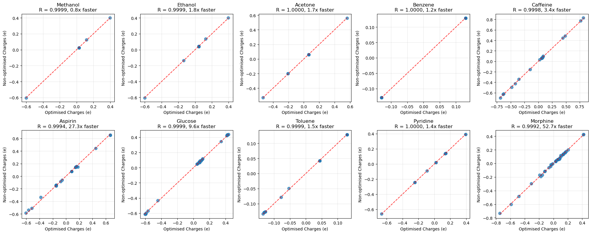
For just this small set of ligands we saved two minutes of computational time accounting for 98.6% of the total computation time; with little effect on the accuracy of the partial charges.
Below are the similarity plots of the charges for each molecule. As we have shown, the non-optimised and optimised AM1BCC charges are very similar.
Conclusion
Setting maxcyc=0 in the SQM settings for antechamber results in a significant speed improvement with little effect on accuracy (on average)
For most drug discovery workflows with pre-optimised structures, geometry optimisation is unnecessary overhead. Use fast mode when:
- Input geometries are well-prepared (RDKit/Schrodinger/MOE)
- Processing large compound libraries
- Doing screening calculations
- Speed matters more than 0.1% accuracy
Use slow mode when:
- Poor input geometries
- Problematic molecules (unusual geometries/charges)
Bottom line: Start with fast mode. Only use slow mode if you encounter problems.