T>T: Order from Chaos: Langton's Ant
Try the code yourself!
Click the following button to launch an ipython notebook on Google Colab which implements the code developed in this post:
![]()
Langton’s Ant
The inspiration for this post came from Numberphile who made a very informative video on a mathematical simulation called Langton’s ant, first described by Chris Langton in 1986. I found this problem fascinating and wanted to program it using Python. First lets discuss the problem.
The Rules
Take an ant, sit them down on a large grid of white squares and give them 2 very simple rules to follow:
1) If you are on a white square, turn 90° clockwise, flip the colour of the square, then move forward one square.
2) If you are on a black square, turn 90° anti-clockwise, flip the colour of the square, then move forward one square.
Now our ant knows the rules and if they cooperate they can set off on their journey around the grid. To make this process easier to understand here is a small animation of the first 200 steps taken from Wikipedia.

Our aim is to program this in Python for \(N\)-steps and look at what path our ant takes. To truly understand a problem, you have to implement it yourself.
The Program
There are numerous ways we could program Langton’s ant but we want to keep it simple and use a small animation to simulate the ant’s trajectory. One of the simplest approaches is to treat the initial white grid as a numpy array of 0’s then iterate through the two rules, moving our ant around the grid making sure they are enforced.
First we want to set the size of our white grid and the number of steps we want our ant to take.
1
2
dim = 100 # Dimensions of the square grid
no_ant_steps = 11000 # Number of steps the ant takes
We can then build our square grid of zeros as a numpy array using dim.
1
grid = np.array(np.zeros((dim, dim)))
It will be useful to define a variable which stores the position of our ant which can be updated when looping through the two rules. We will set the initial position of the ant at the midpoint of the grid but any position can be specified.
1
ant_pos = np.array([[int(dim/2)], [int(dim/2)]])
We will now define a direction variable that will hold the information for the current direction our ant is moving.
1
direction = np.matrix([[1], [0]])
In order to program the rotation of the ant, we will use a rotation matrix which for clockwise rotation has the general form
\[ \begin{bmatrix} \cos(\theta) & \sin(\theta)\\
-\sin(\theta) & \cos(\theta) \end{bmatrix} \]
and for anti-clockwise rotation
\[ \begin{bmatrix} \cos(\theta) & -\sin(\theta)\\
\sin(\theta) & \cos(\theta) \end{bmatrix} \]
If you have not used or are unaware of rotation matrices, let’s analyse how the anti-clockwise form works. The trigonometric functions \(\cos(\theta)\) and \(\sin(\theta)\) represent the \(x\) and \(y\) coordinates respectively of a point on a unit circle demonstrated in the following animation.
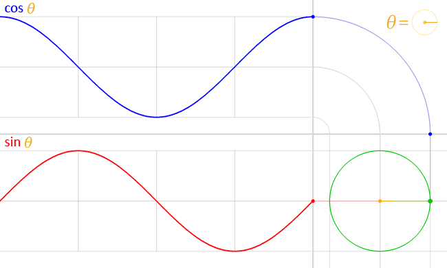
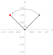
As we move the point around the circumference of the circle, the \(x\) and \(y\) coordinates of the point change inline with \(\cos(\theta)\) and \(\sin(\theta)\). Consider a point in the \(x,y\) plane, with coordinates (1,1). We can rotate this point by 90° anti-clockwise using the transformation matrix as follows
\[ \begin{aligned} \begin{bmatrix} \cos(90) & -\sin(90) \\
\sin(90) & \cos(90) \end{bmatrix} \begin{bmatrix} 1 \\
1 \end{bmatrix} &= \begin{bmatrix} 0 & -1 \\
1 & 0 \end{bmatrix} \begin{bmatrix} 1 \\
1 \end{bmatrix} \\
&= \begin{bmatrix} (0 \times 1) + (-1 \times 1) \\
(1 \times 1) + (0 \times 1) \end{bmatrix} \\
&= \begin{bmatrix} -1 \\
1 \end{bmatrix} \end{aligned} \] We have successfully transformed the point (1,1) to (-1,1) which represents a 90° anti-clockwise rotation around the origin.
We can program these rotation matrices using numpy arrays as follows.
1
2
3
4
# Clockwise rotation matrix
clockwise_rot     = np.array([[0, 1], [-1, 0]])
# Anti-clockwise rotation matrix
anticlockwise_rot = np.array([[0, -1], [1, 0]])
We now define a function which will control the movement of the ant given the two rules it has been told. It will check the colour of the square and invert it, and change the direction of the ant by rotating it. The whole python function will be given first and analysed afterwards, note the comments describe what each part does.
1
2
3
4
5
6
7
8
9
10
11
12
13
14
15
16
17
18
19
20
21
22
23
24
25
26
27
def move_ant(grid, ant_pos, direction):
    '''
    Controls the movement of the ant by a single square

    This function takes the current position and the direction of the ant and updates it via the 2 rules specified above as it takes its next stdep. It then updates the new position, direction and square colour for the next step.

    Parameters:
    grid (np.array)     : This is the grid of dimension, dim, that the ant moves around on
    ant_pos (np.array)  : This represents the ants' position defined as a numpy array of its x,y coordinate on the grid
    direction(np.matrix) : This represents the direction that the ant will move in on this step.

    Returns:
    None: No explicit return
    '''
    # Update the position of the ant
    ant_pos[:] = ant_pos + direction

    # if the ant hits the side of the grid, exit the program
    if any(i == dim or i == 0 for i in ant_pos):
        print("Hit the edge of the board!")
        exit()
    elif grid[ant_pos[0, 0], ant_pos[1, 0]] == 0: # If the ant lands on a white square
        grid[ant_pos[0, 0], ant_pos[1, 0]] = 1 # Change the square from white (0) to black (1)
        direction[:] = clockwise_rot * direction # As it landed on a white square, update the direction with a clockwise rotation
    else: # if the ant lands on a black square
        grid[ant_pos[0, 0], ant_pos[1, 0]] = 0 # Change the square from black (1) to white (0)
        direction[:] = anticlockwise_rot * direction # As it landed on a black square, update the direction with a anti-clockwise rotation
The first thing we do is check that the ant has not hit the side of the grid. There are different ways to handle this exception, but in this instance we are going to initialise the program with a sizeable starting grid and if our ant does hit the side then the program will exit as the ant has escaped! We use the any function in Python which analyses the position indices and checks if any are equal to the lower and upper dimensions of the grid.
1
2
3
4
# if the ant hits the side of the grid, exit the program
if any(i == dim or i == 0 for i in ant_pos):
    print("Hit the edge of the board!")
    exit()
Next we program in rules (1) and (2) which the ant has to follow. The first elif statement controls what happens if the ant lands on a white square and the final else statement controls what happens if the ant lands on a black square.
1
2
3
4
5
6
elif grid[ant_pos[0, 0], ant_pos[1, 0]] == 0: # If the ant lands on a white square
    grid[ant_pos[0, 0], ant_pos[1, 0]] = 1 # Change the square from white (0) to black (1)
    direction[:] = clockwise_rot * direction # As it landed on a white square, update the direction with a clockwise rotation
else: # If the ant lands on a black square
    grid[ant_pos[0, 0], ant_pos[1, 0]] = 0 # Change the square from black (1) to white (0)
    direction[:] = anticlockwise_rot * direction # As it landed on a black square, update the direction with a anti-clockwise rotation
The main part of the program is now complete and we can begin the animation using FuncAnimation from matplotlib. First we create a figure object.
1
2
fig = plt.figure()
ax = fig.add_subplot(111)
Next we use the function imshow to display the image of the grid on a 2D regular raster (A raster is a dot matrix data structure that represents a generally rectangular grid of pixels). cmap represents the colour map which we set as black and white, and vmin and vmax define the data range that the colormap covers i.e. it is a binary colour map, white = 0 and black = 1.
1
im = plt.imshow(a, interpolation='none', cmap='Greys', vmin=0, vmax=1)
Next we define our animate function which we can pass to the FuncAnimation function from matplotlib.
1
2
3
4
5
6
7
8
9
10
11
12
13
14
15
16
def animate_ant(x):
    '''
    This function allows for animation of the move_ant function

    Parameters:
    x : This is a dummy variable only required internally by matplotlib. In the documentation is specifies "The first argument will be the next value in frames." The animating function needs to take an argument, which it generated by whatever frames is set to.

    Returns:
    [Im] : Iterable list, the information required to print the next frame.
    '''
    # Execute the moveant function
    move_ant(grid, ant_pos, direction)
    # Update the grid information for the next frame used in the animation
    im.set_data(grid)
    # Return the information required to print the next frame
    return [im]
(Optional) we now hide the \(x\) and \(y\) axes and save the animation to file.
1
2
3
4
5
6
# Hide the x axis ticks and labels
ax.axes.xaxis.set_visible(False)
# Hide the y axis ticks and labels
ax.axes.yaxis.set_visible(False)
# Save the animation as .mp4
anim.save('Langtons_ant.mp4', writer='ffmpeg')
Now we can collect all of this into one complete program.
The Complete Program
1
2
3
4
5
6
7
8
9
10
11
12
13
14
15
16
17
18
19
20
21
22
23
24
25
26
27
28
29
30
31
32
33
34
35
36
37
38
39
40
41
42
43
44
45
46
47
48
49
50
51
52
53
54
55
56
57
58
59
60
61
62
63
64
65
66
67
68
69
70
71
72
73
74
75
import numpy as np
from matplotlib import pyplot as plt
from matplotlib import animation

# Set the dimensions of the grid
dim = 100
# Set the number of steps the ant should take
ant_steps = 11000
# Build a corresponding numpy array of dimensions (dim,dim)
grid = np.array(np.zeros((dim, dim)))
# Define a variable to represent the current ant_position of the ant on the board
ant_pos = np.array([[int(dim/2)], [int(dim/2)]])
# Define a variable to represent the direction ant is currently moving
direction = np.matrix([[1], [0]])

# Rotation matrix
clockwise_rot     = np.array([[0, 1], [-1, 0]])
anticlockwise_rot = np.array([[0, -1], [1, 0]])
def move_ant(grid, ant_pos, direction):
    '''
    Controls the movement of the ant by a single square

    This function takes the current position and the direction of the ant and updates it via the 2 rules specified above as it takes its next stdep. It then updates the new position, direction and square colour for the next step.

    Parameters:
    grid (np.array)     : This is the grid of dimension, dim, that the ant moves around on
    ant_pos (np.array)  : This represents the ants' position defined as a numpy array of its x,y coordinate on the grid
    direction(np.matrix) : This represents the direction that the ant will move in on this step.

    Returns:
    None: No explicit return
    '''
    ant_pos[:] = ant_pos + direction

    if any(i == dim or i == 0 for i in ant_pos):
        print("Hit the edge of the board!")
        exit()
    elif grid[ant_pos[0, 0], ant_pos[1, 0]] == 0:  # landed on white
        grid[ant_pos[0, 0], ant_pos[1, 0]] = 1 # As landed on white square, change to black square
        direction[:] = clockwise_rot * direction
    else:
        grid[ant_pos[0, 0], ant_pos[1, 0]] = 0
        direction[:] = anticlockwise_rot * direction

fig = plt.figure()
ax = fig.add_subplot(111)
im = plt.imshow(grid, interpolation='none', cmap='Greys', vmin=0, vmax=1)

def animate_ant(x):
    '''
    This function allows for animation of the move_ant function

    Parameters:
    x : This is a dummy variable only required internally by matplotlib. In the documentation is specifies "The first argument will be the next value in frames." The animating function needs to take an argument, which it generated by whatever frames is set to.

    Returns:
    [Im] : Iterable list, the information required to print the next frame
    '''
    # Execute the moveant function
    move_ant(grid, ant_pos, direction)
    # Update the grid information for the next frame used in the animation
    im.set_data(grid)
    # Return the information required to print the next frame
    return [im]

anim = animation.FuncAnimation(fig, animate_ant,
                               frames=ant_steps, interval=20, blit=True,
                               repeat=False)

# Hide the x axis ticks and labels
ax.axes.xaxis.set_visible(False)
# Hide the y axis ticks and labels
ax.axes.yaxis.set_visible(False)

anim.save('Langtons_ant.mp4', writer='ffmpeg')
Program Output
Let us now run our completed Langton’s ant program and see what our little ant does.
Analysis of Results
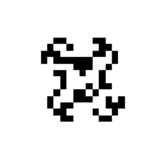
For the first few hundred steps our pioneer ant produces patterns which have crude symmetries and structure such as the following.
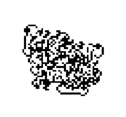
It quickly descends into chaos with no inherent structure or order as our ant follows a psuedo-random path.
However, after our tired ant has completed approximately 10000 steps something interesting happens; order is restored out of chaos.
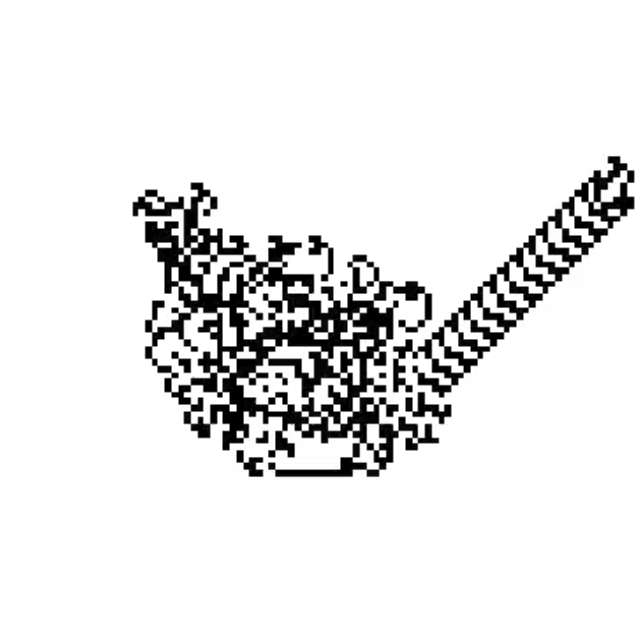
Our ant begins to construct a ‘highway’ pattern that repeats indefinitely. In Chaos theory, a chaotic system is extremely sensitive to its starting conditions; but one of the emergent behaviours of Langton’s Ant is that no matter the pattern of black and white squares at the start the highway structure will always emerge eventually.
What I found fascinating about this simulation is that two very simple rules can lead to such a regular pattern emerging from a seemingly chaotic system. Further T>T posts will explore this in greater details with more variants, initial conditions and number of ants, or experiment with the program yourself!