T>T: From Grid to Gaussian: Accelerating Molecular Similarity Calculations
Try the code yourself!
Click the following button to launch an ipython notebook on Google Colab which implements the code developed in this post:
![]()
The Problem
In computational chemistry, calculating molecular electrostatic potentials, the electric potential energy experienced by a unit positive charge at any point in the space surrounding a molecule, is a common yet computationally intensive task. These potentials often involve evaluating terms like $1/r$, where $r$ is the distance from an atomic centre. Although simple in form, the sheer number of evaluations required often in the millions during molecular similarity or docking workflows can impose a significant computational burden.
Having worked extensively with electrostatic and shape-based similarity methods, I recently revisited this nice paper by Good, Hodgkin, and Richards. The authors demonstrate a surprisingly effective technique: approximating the $1/r$ function using a small number (just two or three) of Gaussian functions. Despite the markedly different form of Gaussians compared to $1/r$, the approximation is impressively accurate. For anyone who has worked in this field, you know how prevalent and foundational Gaussian functions are in computational chemistry; so little tricks such as this can have a surprising impact on numerous problems.
The Mathematical Foundation
The key result from the paper is that any $1/r$ function can be approximated as a sum of Gaussian functions
\[\frac{1}{r} \approx \sum\limits_{i=1}^{n} a_i \text{e}^{-b_ir^2},\]where:
- $a_i$ are the amplitude coefficients
- $b_i$ are the exponential decay parameters
- $n$ is the number of Gaussian functions
They used least-squares fitting to determine the optimal parameters and found the following, 2 and 3-term Gaussian function approximations.
Two-Gaussian approximation
\[\frac{1}{r} \approx 0.2181\text{e}^{-0.0058r^2} + 1.0315\text{e}^{-0.2890r^2}\]Three-Gaussian approximation
\[\frac{1}{r} \approx 0.3001\text{e}^{-0.0499r^2} + 0.9716 \text{e}^{-0.5026 r^2} + 0.1268 \text{e}^{-0.0026 r^2}\]Lets visualise them.
Implementation and Visualisation
Let’s visualise them to see how well they approximate $1/r$ . To do this we will use matplotlib and numpy with a sprinkle of seaborn for some style.
1
2
3
4
5
6
7
8
9
10
11
12
13
14
15
16
17
18
19
20
21
22
23
24
25
26
27
28
29
30
31
32
33
34
35
36
37
38
39
40
41
42
43
44
45
import numpy as np
import matplotlib.pyplot as plt
import seaborn as sns

sns.set_style("dark_grid")

def exact_function(r):
    """Exact 1/r function"""
    return np.where(r == 0, np.inf, 1.0 / r)

def two_gaussian_approx(r):
    """Two-Gaussian approximation to 1/r"""
    a1, b1 = 0.2181, 0.0058
    a2, b2 = 1.0315, 0.2890
    return a1 * np.exp(-b1 * r**2) + a2 * np.exp(-b2 * r**2)

def three_gaussian_approx(r):
    """Three-Gaussian approximation to 1/r"""
    a1, b1 = 0.3001, 0.0499
    a2, b2 = 0.9716, 0.5026
    a3, b3 = 0.1268, 0.0026
    return (a1 * np.exp(-b1 * r**2) +
            a2 * np.exp(-b2 * r**2) +
            a3 * np.exp(-b3 * r**2))

# create distance array
r = np.linspace(0.1, 10, 1000)

# calculate functions
exact = exact_function(r)
two_gauss = two_gaussian_approx(r)
three_gauss = three_gaussian_approx(r)

# create the plot
plt.figure(figsize=(12, 8))
plt.plot(r, exact, 'k-', linewidth=2, label='Exact 1/r')
plt.plot(r, two_gauss, 'r--', linewidth=2, label='2-Gaussian Approximation')
plt.plot(r, three_gauss, 'b:', linewidth=2, label='3-Gaussian Approximation')
plt.xlabel('Distance r')
plt.ylabel('Function Value')
plt.title('Gaussian Approximation to 1/r Function')
plt.legend()
plt.grid(True, alpha=0.3)
plt.ylim(0, 2)
plt.show()
Running this results in the following plot.
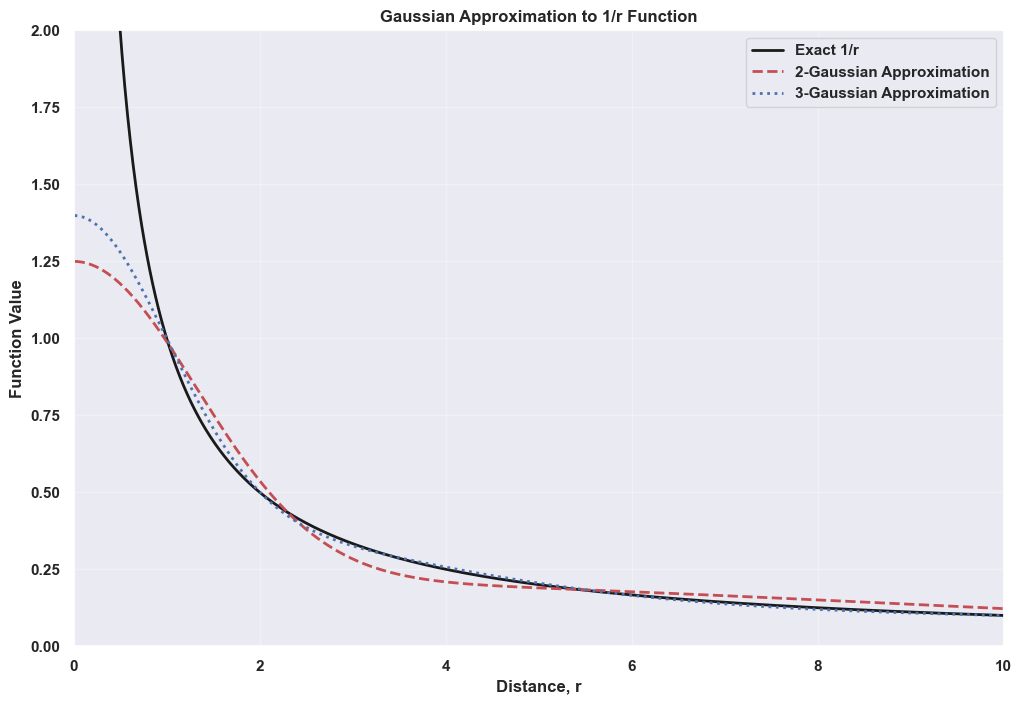
The approximations might look imperfect at first glance, but let’s examine the relative error.
1
2
3
4
5
6
7
8
9
10
11
12
13
14
15
16
17
18
19
20
21
22
23
24
25
26
27
28
def calculate_relative_error(exact, approx):
    """Calculate relative error between exact (1/r) and approximate (2,3 term Gaussians) functions"""
    return np.abs(exact - approx) / exact * 100

# calculate errors
error_2gauss = calculate_relative_error(exact, two_gauss)
error_3gauss = calculate_relative_error(exact, three_gauss)

# plot errors
plt.figure(figsize=(12, 6))
plt.subplot(1, 2, 1)
plt.plot(r, error_2gauss, 'r-', linewidth=2)
plt.xlabel('Distance r')
plt.ylabel('Relative Error (%)')
plt.title('2-Gaussian Approximation Error')
plt.grid(True, alpha=0.3)
plt.ylim(0, 20)

plt.subplot(1, 2, 2)
plt.plot(r, error_3gauss, 'b-', linewidth=2)
plt.xlabel('Distance r')
plt.ylabel('Relative Error (%)')
plt.title('3-Gaussian Approximation Error')
plt.grid(True, alpha=0.3)
plt.ylim(0, 20)

plt.tight_layout()
plt.show()
Which produces the following two plots.
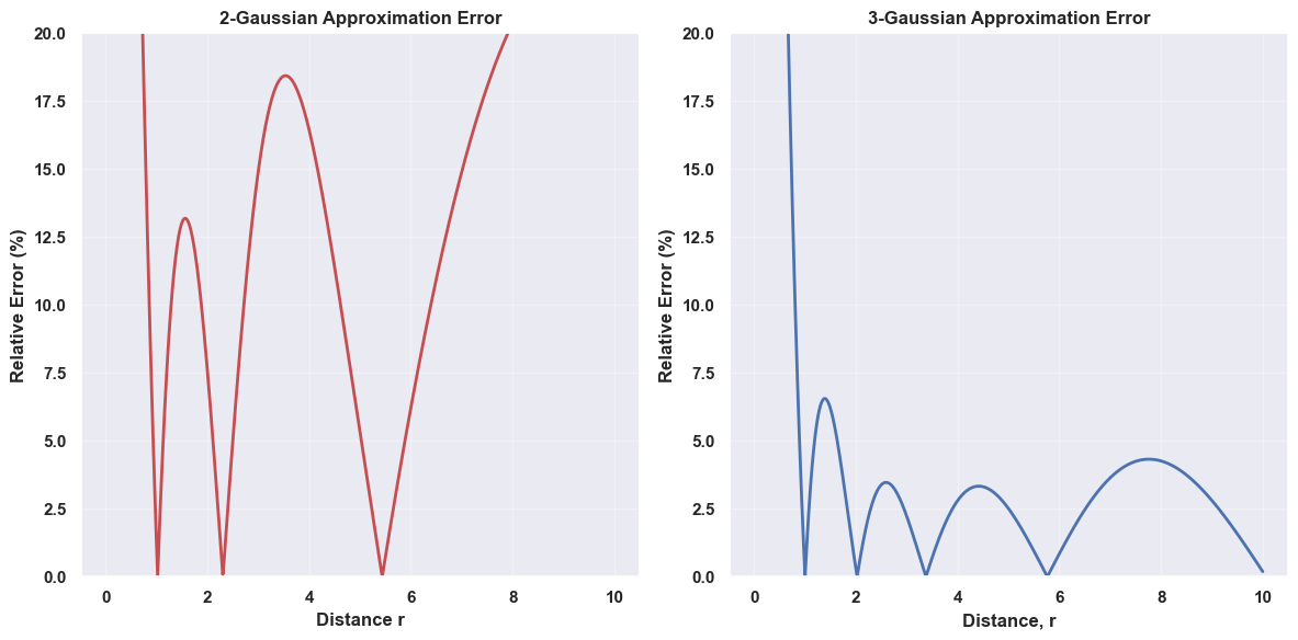
Both approximations have the largest error around $r=0$, where the Gaussian functions cannot replicate the asymptotic behavior of $1/r$. However, this is precisely where the approximation matters least in practical applications in drug discovery.
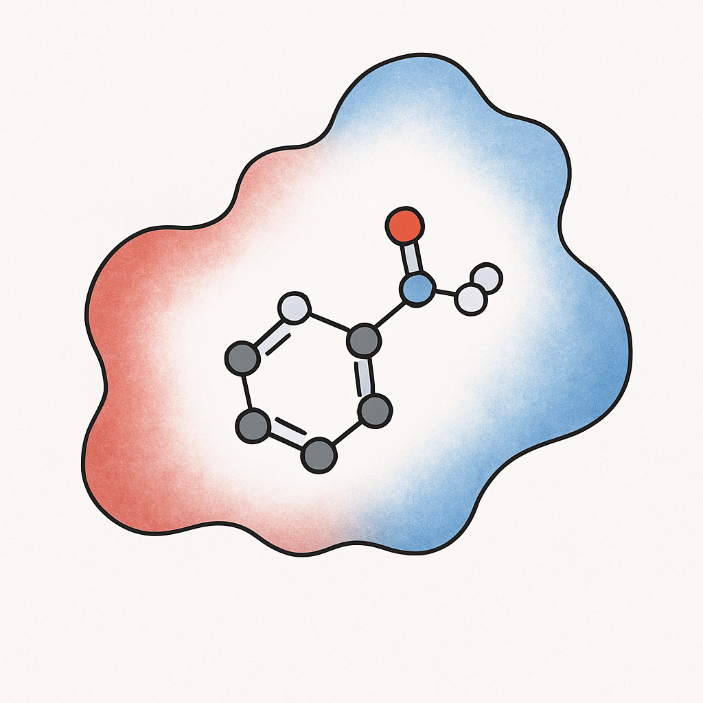
Consider the use-case where we are looking to calculate the electrostatic similarity between two molecules $A$ and $B$, i.e., how alike they are by comparing the spatial distribution of their electric fields, essentially measuring whether they would interact with other molecules in similar ways. The Coulomb potential $V(r)$ describes the electric potential at a point $r$ as a sum of potentials of point charges $q_i$ at points $r_i$ as
\(V(r) = \frac{1}{4\pi \epsilon_0}\sum\limits_{i}\frac{q_i}{|r - r_i|},\) where $\epsilon_0$ is the vacuum permittivity. Analytic integration of the Coulomb potential at $r=0$ is not possible so we turn to our 2 and 3-term Gaussian approximations. In electrostatic similarity calculations, the primary focus lies on the molecular surface rather than the behavior of the Coulomb potential near the atomic nuclei. This is because the region of chemical interaction is effectively defined by the van der Waals radii of the constituent atoms. Therefore, in computational models, the asymptotic behavior of the Coulomb potential near the nucleus is of little concern as it is the potential around the van der Waals surface that governs electrostatic similarity and molecular recognition. See the image below for a representation of an electrostatic potential surface for a drug-like molecule.
This is why these approximations work well, we are not concerned about the chemical physics in the region where the two approximations have the greatest error. Looking at the relative error plot above for the 3-Gaussian approximation, past a distance of $r \approx 1.5$, the relative error drops to $<4\%$ which is certainly accurate for molecular similarity calculations.
Hopefully we are now happier with the notion of approximating a $1/r$ function using 2 or 3 Gaussian functions. We will now explore the electrostatic similarity use-case further to emphasise the advantages these kinds of approximations offer.
Use in Computational Chemistry
In molecular similarity calculations, we need to evaluate integrals of the form
\[\int\int\int V_A(r)V_B(r) \text{d}V,\]where $V_A$ and $V_B$ are the electrostatic potentials of molecules $A$ and $B$. Without a functional approximation we would normally need to turn to some sort of grid-based technique or Monte Carlo style integration which are slower and often present convergence issues.
When these potentials are expressed using Gaussian functions, these integrals become analytical and extremely fast to compute without convergence issues. Let’s implement both methods to see the difference in computational performance. We are going to calculate the electrostatic similarity using the Carbo similarity index
\[S_{AB} = \frac{\int\int\int V_A(r) V_B(r) \text{d}V}{\left(\int\int\int V_A^2(r)\right)^{\frac{1}{2}} \left(\int\int\int V_B^2(r)\right)^{\frac{1}{2}} }.\]This formula computes the normalised overlap between two molecular electrostatic potential fields. The numerator represents the cross-correlation between the potentials, while the denominator normalises by the magnitude of each potential field.
Method 1: Traditional Grid-Based Method
A conventional approach requires numerical integration over a three-dimensional grid. The key steps are:
1
2
3
4
5
6
7
8
9
10
11
12
13
14
15
16
17
18
19
20
21
22
23
24
25
26
27
28
29
30
31
32
33
34
35
36
37
38
39
40
41
42
43
44
45
def grid_similarity(charges_A, coords_A, charges_B, coords_B,
                   grid_spacing=1.0, grid_extent=4.0):
    """
    Calculate similarity using grid-based numerical integration
    """
    import time
    start_time = time.perf_counter()

    # Step 1: Determine grid boundaries
    all_coords = np.vstack([coords_A, coords_B])
    min_coords = np.min(all_coords, axis=0) - grid_extent
    max_coords = np.max(all_coords, axis=0) + grid_extent

    # Step 2: Generate grid points
    x = np.arange(min_coords[0], max_coords[0] + grid_spacing, grid_spacing)
    y = np.arange(min_coords[1], max_coords[1] + grid_spacing, grid_spacing)
    z = np.arange(min_coords[2], max_coords[2] + grid_spacing, grid_spacing)

    X, Y, Z = np.meshgrid(x, y, z, indexing='ij')
    grid_points = np.column_stack([X.ravel(), Y.ravel(), Z.ravel()])
    n_points = len(grid_points)

    # Step 3: Calculate electrostatic potential for both molecules
    V_A = np.zeros(n_points)
    for q, coord in zip(charges_A, coords_A):
        distances = np.linalg.norm(grid_points - coord, axis=1)
        distances = np.maximum(distances, 0.1)  # Avoid singularities
        V_A += q / distances

    V_B = np.zeros(n_points)
    for q, coord in zip(charges_B, coords_B):
        distances = np.linalg.norm(grid_points - coord, axis=1)
        distances = np.maximum(distances, 0.1)
        V_B += q / distances

    # Step 4: Numerical integration
    volume_element = grid_spacing ** 3
    numerator = np.sum(V_A * V_B) * volume_element
    denom_A = np.sum(V_A * V_A) * volume_element
    denom_B = np.sum(V_B * V_B) * volume_element

    similarity = numerator / np.sqrt(denom_A * denom_B)
    computation_time = time.perf_counter() - start_time

    return similarity, computation_time, n_points
Computational Complexity: $O(N \times M \times P)$ where $N$ and $M$ are the number of atoms, and $P$ is the number of grid points. For a typical grid with 100,000 points, this becomes very computationally expensive.
Method 2: Gaussian Approximation
Now let’s implement the Gaussian approach, which replaces numerical integration with analytical calculations.
1
2
3
4
5
6
7
8
9
10
11
12
13
14
15
16
17
18
19
20
21
22
23
24
25
26
27
28
29
30
31
32
33
34
35
36
37
38
39
40
41
42
43
44
45
46
47
48
def gaussian_similarity(charges_A, coords_A, charges_B, coords_B, method='two_gaussian'):
    """
    Calculate similarity using Gaussian approximation with analytical integration
    """
    import time
    start_time = time.perf_counter()

    # Define Gaussian parameters from the 1992 paper
    gaussian_params = {
        'two_gaussian': [(0.2181, 0.0058), (1.0315, 0.2890)],
        'three_gaussian': [(0.3001, 0.0499), (0.9716, 0.5026), (0.1268, 0.0026)]
    }
    params = gaussian_params[method]

    def gaussian_overlap_integral(q1, r1, q2, r2, a, b):
        """
        Analytical integral of two Gaussian functions

        For two Gaussians centered at r1 and r2 with charges q1 and q2,
        the overlap integral has a closed-form solution
        """
        r_diff_sq = np.sum((r1 - r2)**2)
        return q1 * q2 * a * (np.pi / b)**(3/2) * np.exp(-b * r_diff_sq)

    # Calculate numerator (cross-correlation)
    numerator = 0
    for qa, ra in zip(charges_A, coords_A):
        for qb, rb in zip(charges_B, coords_B):
            for a, b in params:
                numerator += gaussian_overlap_integral(qa, ra, qb, rb, a, b)

    # Calculate normalization terms
    denom_A = 0
    for qa1, ra1 in zip(charges_A, coords_A):
        for qa2, ra2 in zip(charges_A, coords_A):
            for a, b in params:
                denom_A += gaussian_overlap_integral(qa1, ra1, qa2, ra2, a, b)

    denom_B = 0
    for qb1, rb1 in zip(charges_B, coords_B):
        for qb2, rb2 in zip(charges_B, coords_B):
            for a, b in params:
                denom_B += gaussian_overlap_integral(qb1, rb1, qb2, rb2, a, b)

    similarity = numerator / np.sqrt(denom_A * denom_B)
    computation_time = time.perf_counter() - start_time

    return similarity, computation_time
Computational Complexity: $O(N \times M \times G)$ where $G$ is the number of Gaussian terms (2 or 3). This is dramatically more efficient than grid-based methods.
Method 3: optimised vectorised Implementation
The nested loops in Method 2 are inefficient in Python. Let’s vectorize using NumPy operations:
1
2
3
4
5
6
7
8
9
10
11
12
13
14
15
16
17
18
19
20
21
22
23
24
25
26
27
28
29
30
31
32
33
34
35
36
37
38
39
40
41
42
43
44
45
def optimised_gaussian_similarity(charges_A, coords_A, charges_B, coords_B, method='two_gaussian'):
    """
    optimised Gaussian similarity using vectorised operations
    """
    import time
    from scipy.spatial.distance import cdist
    start_time = time.perf_counter()

    gaussian_params = {
        'two_gaussian': [(0.2181, 0.0058), (1.0315, 0.2890)],
        'three_gaussian': [(0.3001, 0.0499), (0.9716, 0.5026), (0.1268, 0.0026)]
    }
    params = gaussian_params[method]

    def optimised_gaussian_integral(dist_matrix, charges1, charges2):
        """vectorised Gaussian integral calculation"""
        integral = 0.0

        for a, b in params:
            # vectorised exponential calculation
            exp_term = np.exp(-b * dist_matrix**2)

            # Broadcasting for charge products
            charge_products = charges1[:, np.newaxis] * charges2[np.newaxis, :]

            # vectorised contribution calculation
            contribution = a * (np.pi / b)**(3/2) * charge_products * exp_term
            integral += np.sum(contribution)

        return integral

    # Precompute all pairwise distance matrices
    dist_AA = cdist(coords_A, coords_A)
    dist_AB = cdist(coords_A, coords_B)
    dist_BB = cdist(coords_B, coords_B)

    # Calculate all required integrals
    integral_AA = optimised_gaussian_integral(dist_AA, charges_A, charges_A)
    integral_AB = optimised_gaussian_integral(dist_AB, charges_A, charges_B)
    integral_BB = optimised_gaussian_integral(dist_BB, charges_B, charges_B)

    similarity = integral_AB / np.sqrt(integral_AA * integral_BB)
    computation_time = time.perf_counter() - start_time

    return similarity, computation_time
Performance improvements:
- Eliminates slow Python loops
- Uses vectorised NumPy operations
- Provides additional 2-10x speedup over Method 2
Comparing the Three Approaches
Let’s test all three methods:
1
2
3
4
5
6
7
8
9
10
11
12
13
14
15
16
17
18
19
20
21
22
23
24
25
26
27
28
29
30
31
32
33
34
35
36
def compare_methods():
    """Compare all three methods on the same system"""
    # Simple test system: 3 atoms
    charges = np.array([0.5, -0.25, -0.25])
    coords = np.array([[0.0, 0.0, 0.0], [1.0, 0.0, 0.0], [0.0, 1.0, 0.0]])
    coords_shifted = coords + np.array([2.0, 0.0, 0.0])

    print("Method Comparison:")
    print("=" * 50)

    # Method 1: Grid-based
    sim1, time1, n_points = grid_similarity(
        charges, coords, charges, coords_shifted,
        grid_spacing=0.5, grid_extent=2.0
    )
    print(f"Grid method: {sim1:.6f} ({time1:.6f}s, {n_points:,} points)")

    # Method 2: Basic Gaussian
    sim2, time2 = gaussian_similarity(
        charges, coords, charges, coords_shifted,
        method='two_gaussian'
    )
    print(f"Gaussian method: {sim2:.6f} ({time2:.6f}s)")

    # Method 3: optimised Gaussian
    sim3, time3 = optimised_gaussian_similarity(
        charges, coords, charges, coords_shifted,
        method='two_gaussian'
    )
    print(f"optimised method: {sim3:.6f} ({time3:.6f}s)")

    print(f"\nSpeedups:")
    print(f"Gaussian vs Grid: {time1/time2:.1f}x")
    print(f"optimised vs Grid: {time1/time3:.1f}x")

compare_methods()
This progression shows performance improvements:
- Grid method: High accuracy but expensive O(N×M×P) scaling
- Gaussian method: Analytical integrals reduce complexity to O(N×M×G)
- optimised method: Vectorization provides additional 2-10x speedup (I think…)
Production-Ready Implementation
If I were to use this in a real-world example I would wrap it in a “production-ready” class:
1
2
3
4
5
6
7
8
9
10
11
12
13
14
15
16
17
18
19
20
21
22
23
24
25
26
27
28
29
30
31
32
33
34
35
36
37
38
39
40
41
42
43
44
45
46
47
class ElectrostaticComparison:
    """
    Production-ready class for electrostatic similarity calculations
    """

    def __init__(self):
        self.gaussian_params = {
            'two_gaussian': [(0.2181, 0.0058), (1.0315, 0.2890)],
            'three_gaussian': [(0.3001, 0.0499), (0.9716, 0.5026), (0.1268, 0.0026)]
        }

    def calculate_similarity(self, charges_A, coords_A, charges_B, coords_B,
                           method='optimised', gaussian_type='three_gaussian'):
        """
        Calculate electrostatic similarity between two molecules

        Parameters:
        -----------
        charges_A, charges_B : array-like
            Atomic partial charges
        coords_A, coords_B : array-like
            Atomic coordinates (N×3)
        method : str
            'grid', 'gaussian', or 'optimised'
        gaussian_type : str
            'two_gaussian' or 'three_gaussian'

        Returns:
        --------
        similarity : float
            Carbó similarity index
        time : float
            Computation time in seconds
        """
        if method == 'grid':
            return self.grid_similarity(charges_A, coords_A, charges_B, coords_B)
        elif method == 'gaussian':
            return self.gaussian_similarity(charges_A, coords_A, charges_B, coords_B,
                                          gaussian_type)
        elif method == 'optimised':
            return self.optimised_gaussian_similarity(charges_A, coords_A, charges_B, coords_B,
                                                     gaussian_type)
        else:
            raise ValueError(f"Unknown method: {method}")

    # Include the three methods we defined above as class methods
    # grid_similarity, gaussian_similarity, optimised_gaussian_similarity
Usage Example
Here’s how to use the class in practice:
1
2
3
4
5
6
7
8
9
10
11
12
13
14
15
16
17
18
19
20
21
22
23
24
25
26
# Initialize the comparison class
comp = ElectrostaticComparison()

# Example molecules (water and methanol partial charges/coordinates)
water_charges = np.array([-0.834, 0.417, 0.417])
water_coords = np.array([[0.0, 0.0, 0.1173], [0.0, 0.7572, -0.4692], [0.0, -0.7572, -0.4692]])

methanol_charges = np.array([-0.700, 0.435, 0.435, 0.145, -0.683, 0.418])
methanol_coords = np.array([[-0.748, -0.015, 0.024], [-1.293, 0.202, -0.900],
                            [-1.263, 0.422, 0.856], [-0.882, -1.090, 0.211],
                            [0.716, 0.024, -0.016], [0.957, -0.191, -0.923]])

# Calculate similarity using different methods
sim_grid, time_grid = comp.calculate_similarity(
    water_charges, water_coords, methanol_charges, methanol_coords,
    method='grid'
)

sim_opt, time_opt = comp.calculate_similarity(
    water_charges, water_coords, methanol_charges, methanol_coords,
    method='optimised', gaussian_type='two_gaussian'
)

print(f"Grid method: {sim_grid:.6f} ({time_grid:.4f}s)")
print(f"optimised Gaussian: {sim_opt:.6f} ({time_opt:.6f}s)")
print(f"Speedup: {time_grid/time_opt:.1f}x")
Running the notebook (checkout the button at the top of this page) I get
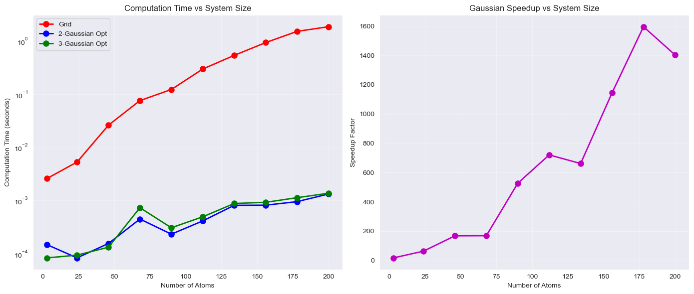
Which demonstrates a remarkable speedup of the 2,3 Gaussian approximations over the grid-based method!
Conclusion
Approximating $1/r$ with a small number of Gaussian functions demonstrates the remarkable versatility of Gaussian basis functions in computational chemistry. Despite their markedly different mathematical form, just two or three parameterised Gaussians can reproduce the $1/r$ behavior with impressive accuracy in the regions that matter most for molecular similarity calculations.
The performance gains are substantial and scale favourably with system size:
- Speed: Gaussian methods provide multiple order of magnitude speedup over grid-based approaches, with larger speedups for bigger systems
- Accuracy: 3-Gaussian approximations maintain <4% error in relevant regions (r > 1.5 Å)
- Scalability: Computational complexity drops from O(N×M×P) to O(N×M×G) where G=2 or 3
- Memory efficiency: Analytical integrals eliminate the need for large grid arrays
- Vectorization: NumPy operations provide additional 2-10x performance improvements
For practical applications in drug discovery and molecular similarity screening, the optimised Gaussian approach offers the best balance of speed, accuracy, and simplicity. Previously I have used these methods for:
- High-throughput virtual screening campaigns
- Molecular database searching and clustering
- Shape and electrostatic complementarity calculations (main application I have worked on)
- Real-time interactive molecular design applications
Gaussian functions provide a powerful mathematical framework for accelerating a wide range of molecular calculations where analytical solutions can replace expensive numerical integrations.
Sometimes the right approximation, carefully chosen, can deliver orders of magnitude performance improvement with negligible accuracy loss. The art lies in understanding your problem well enough to know where precision matters and where it doesn’t (I say this as though it is simple, it is not. A big thrill is when you do understand a problem well enough to unravel it to its core and rebuild it with the fewest moving parts).
References
- Good, A. C., Hodgkin, E. E., & Richards, W. G. (1992). Utilization of Gaussian functions for the rapid evaluation of molecular similarity. Journal of Chemical Information and Computer Sciences, 32(3), 188-191. https://pubs.acs.org/doi/10.1021/ci00007a002