T>T: Surprising Behaviour in the Bond Length of the Hydrogen Molecular Ion
The inspiration for this post came from this paper by J. D. Dunitz and T. K. Ha titled:
By considering the hydrogen molecule, H\(_2\) (2 protons, 2 electrons), they showed that the calculated bond length temporarily decreased as the charge of the nuclei increased. This is a counter intuitive result as like charges repel, so we might think larger magnitude like-charges should exhibit greater repulsion. If we remove one of the electrons to form the hydrogen molecular ion (2 protons, 1 electron), H\(_2^+\), is this behaviour still true?
In this post we answer this question, for I believe, the first time.
Hydrogen Molecular Ion
The hydrogen molecular ion, H\(_2^+\), also referred to as the dihydrogen cation represents the simplest molecular ion in nature, and can be formed from the ionization of the hydrogen molecule, H\(_2\) resulting in a three-particle system consisting of two protons and one electron, artfully depicted below using the graphical finesse of plain text, I spared no expense.
	    e⁻
	   / \
	   /    \
	    p⁺ --- p⁺
H\(_2^+\) holds a significant place in the history of physics as the first application of quantum mechanics to a molecule, predicting a bound state solution where classical mechanics could not.
The complete Schrödinger equation cannot be solved exactly but by invoking the Born-Oppenheimer approximation the electronic Schrödinger equation can be solved exactly using confocal-elliptic coordinates. This allows for complete separation of the Hamiltonian resulting in two coupled differential equations solvable using a recurrence relation.
With the advancement in computer power, we can obtain very accurate energies and wave functions to these molecular ions without assuming the Born Oppenheimer approximation i.e. including the motion of the nuclei explicitly in the calculation. I have previously published work which accomplishes this and in this post we will use these very high accuracy wavefunctions to explore the effect of nuclear charge on the bond length in hydrogen molecular-like ions with different nuclear charges.
How to Calculate Bond Length?
The bond length of H\(_2^+\) is the distance between the two protons, but how do we calculate this distance? Quantum physics textbooks tell us the expected value of a physical quantity corresponds to the measured value from an experiment.
The expectation value corresponds to the average value so can be thought of as an average of all the possible outcomes of a measurement as weighted by their likelihood. Something we found in the paper cited above is that the calculated expectation values of the proton-proton distance did not agree well with the experimental value, whilst the most probable value did. Have a look at the following table which lists the calculated values of \(\langle \Psi \rvert r_3 \rvert \Psi \rangle\) and the most probable value of \(r_3\) for H\(_2^+\) where \(r_3\) is the distance between the two protons.
| \( \langle \Psi \rvert r_3 \rvert \Psi \rangle \) / bohr | Most probable \( r_3 \) / bohr | |
|---|---|---|
| Calculated | 2.063 913 867 | 1.989 685 |
| Experiment\(^{[1]}\) | 1.987 99 | 1.987 99 |
The calculated value of the most probable \(r_3\) agrees with experiment to three significant figures, whilst the expectation value of \(r_3\) agrees to zero significant figures. For the purposes of our investigation we will calculate both of these quantities and see how they compare.
Method
A brief overview of the method used to numerically solve the Schrodinger equation is now given, for a more indepth discussion consult this review paper we published.
Assume the following wavefunction form, consisting of a triple orthogonal set of Laguerre polynomials
\[\Psi (u,v,w) = e^{-\frac{1}{2}(u+v+w)} \times\sum\limits_{l,m,n=0}^{\infty}A(l,m,n) L_{l}(u)L_{m}(v)L_{n}(w),\]where \(u,v,w\) are perimetric coordinates, linear combinations of inter-particle coordinates
\[u = \alpha(r_2+r_{12}-r_1), \ v = \beta(r_1+r_{12}-r_2), \ w= \gamma(r_1+r_2-r_{12}),\]where \(\alpha,\beta,\gamma\) are non-linear variational parameters.
Substitute the wavefunction form into the time independent, non-relativistic Schrödinger equation
\[\left(-\frac{1}{2\mu_{13}}\nabla_1^2 - \frac{1}{2\mu_{23}}\nabla_2^2 -\frac{1}{m_3}\nabla_1\cdot\nabla_2 + \frac{Z_1Z_3}{r_1} + \frac{Z_2Z_3}{r_2} + \frac{Z_1Z_2}{r_{12}}\right)\Psi = E\Psi.\]Substitute the Laguerre recursion relations
\[\begin{align*} xL_n(x) &= -(n+1)L_{n+1}(x) + (2n+1)L_n(x) - nL_{n-1}(x) \\ xL'_n(x) &= nL_n(x) - nL_{n-1}(x) \\ xL''_n(x) &= (x-1)L'_n(x) - nL_n(x) \end{align*}\]Which leads to a 57-term recursion relation
\[\sum\limits_{a,b,c = -2}^{+2}C_{a,b,c}(l,m,n)A(l+a, m+b, n+c) = 0.\]Collapsing the triple index, \(l,m,n\) down results in
\[\sum\limits_{k}^{}C_{ik}B_k = 0.\]Which we solve as a generalized eigenvalue problem
\[\sum\limits_{k}^{}\left(H_{ik} - ES_{ik}\right)B_k = 0,\]where \(B_k\) is the eigenvector (wavefunction).
Modest 2856-term wavefunctions were calculated for hydrogen molecular-like systems with nuclear charges in the range \(0.4 \le Z \le 1.3\) in steps of \(Z = 0.1\) with smaller increments around the dissociation region. The calculated energies were accurate to approximately pico-hartree accuracy and the resultant wavefunctions were then used to calculate the average value of \(r_3\) and the most probable value of \(r_3\). We will now discuss how this is done.
Particle Densities and the Most Probable Bond Distance
Once the wavefunctions, \(\Psi\), have been calculated for all the systems with unique nuclear charge values, \(Z\), they are used to calculate the particle density which more generally between two points \(P\) and \(a_1\) is defined as
\[D_{P,a_1}^{(1)}(\mathbf{R}) = \left\langle\Psi|\delta(\mathbf{x}_{a_1} - \mathbf{x}_{P} - \mathbf{R})|\Psi\right\rangle,\]which characterizes the spatial distribution of particle \(a_1\) with respect to some body-fixed point \(P\) which is chosen here to be \(a_2\) the other proton. For states with angular momentum \(L = 0\) and parity \(p = +1\) the wave function, and thus the particle densities, are spherically symmetric. Therefore \(\mathbf{D}_{P ,a_1}^{(1)} (\mathbf{R})\), \(P = a_2\) are spherically symmetric and their values depend only on the length of \(R\). We now introduce the following
\[\rho_{P, a_1}(r) = \mathbf{D}_{P ,a_1}^{(1)} (\mathbf{R}),\]with, \(\mathbf{R} = (0,0,r)\) and \( r = \lvert\mathbf{R}\rvert \), \( r \in \mathbb{R}_0^+ \). Simplifying all this terminology down gives us the intracule density, \(h(r)\) between the two protons
\[h(r) \equiv \rho_{p^+, p^+}(r) = \left\langle\Psi|\delta(r_3 - r)|\Psi\right\rangle.\]A unique and really interesting property of the Dirac delta function is the sifting property, defined as
\[\int\limits_{-\infty}^{\infty}f(x)\delta(x - x_0)\texttt{d}x = f(x_0),\]and gives the Dirac delta function a sense of measure. It measures the value of \(f(x)\) at the point \(x_0\). This is what the Dirac delta function above is doing, it ‘measures’ the value of \(\Psi\Psi\) at the value \(r\) which allows us to move between the two protons in increments and measure this density at each point resulting in a list of density values which we can then plot. We then take the maximum values of these densities to calculate the most probable bond distance.
In integral form this calculation looks like
\[h(r) = \int\limits_{0}^{\infty}\int\limits_{0}^{\infty}\Psi(r_1,r_2,r)\Psi(r_1,r_2,r)\texttt{d}r_2\texttt{d}r_1\large\rvert_{r_3 = r}\]The calculation itself uses parallelized numerical integration in C++. I will describe how to do this in a future post.
Expectation Value of \(r_3\)
We described above how to calculate the particle density in order to find the most probable bond distance, but how do we calculate the expectation value? This is done using the following
\[\left\langle \Psi|r_3|\Psi\right\rangle = \int\limits_{0}^{\infty}\int\limits_{0}^{\infty}\int\limits_{|r_1-r_2|}^{|r_1+r_2|}\Psi(r_1,r_2,r_3)\Psi(r_1,r_2,r_3)\texttt{d}r_3\texttt{d}r_2\texttt{d}r_2,\]where coordinate transformations are applied to convert the inter-particle coordinates, \(r_1, r_2, r_3\) into the perimetric coordinate counterparts, \(u, v, w\) which removes the triangular condition in the integration and results in independent integration domains ranging between 0 and \(\infty\).
The calculation itself can use the same parallelized numerical integration code mentioned above but can also be solved using the Laguerre recursion relations. This topic, given its depth and tangential nature, might find its place in a future blog post, where a more in-depth exploration can be undertaken.
Results
The following table shows the calculated expectation value (average value) and most probable value of \(r_3\) between the two protons with nuclear charges in the range \(0.4 \le Z \le 1.3\). Why 1.3? when the charge of the two ‘protons’ is 1.3, the system is unbound, shown by the sudden increase in bond length from approximately 2 bohr to > 140 bohr. Physically this means the electron no longer has the influence to hold the two protons in a bound state.
| Nuclear charge / Z | \( \langle \Psi \rvert r_3 \rvert \Psi \rangle \) / bohr | \(4\pi r^2 \Psi \Psi_{\texttt{max}}\) / bohr |
|---|---|---|
| 0.4 | 2.296 558 484 | 2.260 134 |
| 0.5 | 2.158 214 212 | 2.125 930 |
| 0.6 | 2.078 038 239 | 2.048 665 |
| 0.7 | 2.035 824 320 | 2.007 950 |
| 0.8 | 2.021 769 795 | 1.994 954 |
| 0.9 | 2.031 411 074 | 2.004 474 |
| 1.0 | 2.063 913 867 | 2.035 328 |
| 1.1 | 2.122 205 373 | 2.092 229 |
| 1.2 | 2.215 691 763 | 2.185 469 |
| 1.21 | 2.228 968 027 | 2.202 792 |
| 1.22 | 2.241 708 265 | 2.212 782 |
| 1.23 | 2.255 127 463 | 2.227 767 |
| 1.24 | 2.269 180 307 | - |
| 1.241 | 2.270 636 718 | - |
| 1.242 | 2.272 101 112 | - |
| 1.243 | 42.561 145 435 | - |
| 1.3 | 141.428 426 211 | - |
Note that in the particle densities a spherical average was applied, \(4\pi r^2\), which changes the numerical values when compared to those presented in the first table but does not affect the trend or turning point. You will notice that there are values missing in the above table fgor the most probable bond lengths for \(Z > 1.23\) and this is because these values were not calculatable, owing to the system dissociating and the density becomes incredibly diffuse over all space.
Note The values for the maximum positions in the particle densities were calculated through interpolation of the particle density data points using a spline fitting. This is so we do not need to calculate thousands of data points, instead requring fewer and can ‘fill in’ the gaps using a good quality spline fit and differentiate this function to find the maximum. The plot below shows the expectation value and most probable bond lengths against nuclear charge.
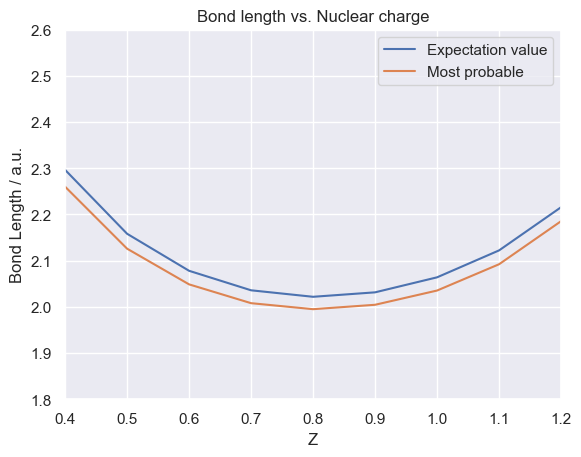
The bond length can be seen to decrease as the nuclear charge increases between \( 0.4 < Z < 0.9 \) where it then begins to increase up to \(Z=1.243\) where the system becomes unbound. The turning point is at \(Z=0.9\)
By just considering the two protons the result seems counter-intuitive, but the presence of the electron explains the physics behind this behaviour. The electron has a charge of -1 so when the nuclear charges of the protons are < 1 the electron dominates the electrostatic interactions in the system. Even though the mass of the proton is ~ 1836 times greater than the mass of the electron, it is able to localize the protons to be closer together via its charge influence. As the charge of the protons increases to \(Z=0.9\) the charge advantage the electron had is now diminished where the dominance shifts to the protons which have a much higher mass and now comparable charge.
To finish off lets have a look at what the particle density does as the nuclear charge increases, which has been visualised in the following animation. The vertical dotted line represents the most probable bond length (with spherical average) for the hydrogen molecular ion, H\(_2^+\). The path of the maximum position is traced out to give you a better understanding of how it changes with charge.
This is a really nice way to visualise how the particle density changes with increasing nuclear charge:
We can see that when the charge of the protons is \(Z=0.4\) the particle density profile is wider which signifies a greater uncertainty in the bond length as it has a greater probability of exisiting over a wider space, \(r\).
As the charge increases further, the particle density profile becomes narrower and taller which signifies the uncertainty in bond length is decreasing: the increased charge is stabilising the system.
At the end of the animation it looks like the plots dissapear but they do not. At \(Z=1.24\) there is a dramatic change in the particle density as the system becomes unbound into a hydrogen atom and a lone electron which means the density becomes massively diffuse over all space. The scales change by orders of magnitude and so it collapses to the axis in the above animation which is just visible.
Conclusions
We have shown that the bond length in H\(_2^+\) temporarily decreases as the charge of the nuclei increases which is exactly what J. D. Dunitz and T. K. Ha showed in their paper for the hydrogen molecule, \(H_2\). It took a bit of work getting there but it is really nice to verify their result for the hydrogen molecular ion and to discover some really interesting quantum physics along the way.
References
[1] Taken from NIST