Try the code yourself!

Click the following button to launch an ipython notebook on Google Colab which implements the code developed in this post:

What is Brownian Motion?

Brownian motion named after its discoverer, botanist Robert Brown, is the motion exhibited by a small particle totally immersed in a liquid or gas. It is an example of a stochastic process, referring to a family of random variables indexed against some other variable or set of variables. Stochastic processes are used as mathematical models of systems appearing to vary in a random manner such as:

• Growth of a bacterial population,
• Decay of radioactive elements,
• Movement of a gas molecule,

With Brownian motion being one of the most useful stochastic processes in applied probability theory. We are going to simulate a gas molecule moving around a 3-dimensional box using NumPy and matplotlib. First lets cover the maths required to model the random motion of our gas molecule, it ends up being much simpler than it looks!

Mathematics

A stochastic process, \(X(t)\), is said to be a Brownian motion process if\(^{[1]}\):

• \(X(0)=0\) is certain, i,e, has probability 1.
• \(\lbrace X(t), t \ge 0\rbrace \) has stationary and independant increments.
• For every \(t>0\), \(X(t)\) is normally distributed with mean, \(\mu = 0\) and variance \(\sigma^2 = 1\).

\[ \begin{aligned} X(t_2) - X(t_1) &\approx \sqrt{t_2 - t_1}\mathcal{N}(\mu,\sigma^2)
dX(t_i) &\approx \sqrt{\Delta t}\mathcal{N}(0,1) \end{aligned} \tag{1} \] where \(\mathcal{N}(\mu,\sigma^2)\) denotes the normal distribution. In order to simulate this in Python, we need to start by discretizing our time interval \([0,T]\) into \(N\) time steps, \(\Delta t\):

1
2
3
4
5
6
7
8
9
10
11
12

import numpy as np 
import matplotlib.pyplot as plt
from matplotlib.animation import FuncAnimation # call the animation module of matplotlib
from IPython.display import HTML               # this is only required when running the code in the Jupyter notebook
import mpl_toolkits.mplot3d.axes3d as p3       # this imports the 3d axis option from matplotlib otherwise we only have access to 2d space! 

fig = plt.figure()
ax = p3.Axes3D(fig)

T = 1    # this is an arbitrary time unit
N = 1000 # number of steps
dt = T/N # the ratio gives the time step increment

We initiate the figure object using plt.figure() from matplotlib but in this instance we initialise the axis object as a 3d axis object using p3.Axes3D(fig) which tells matplotlib to accept and display \(x, y, z\) data to form a 3D plot.

As our as molecule is moving inside a box we need to know its \(x\), \(y\) and \(z\) coordinates in order to map its path as it moves through the box. Equation (1) shows us that this is just the product of the square root of the time interval, \(\Delta t\) and a random number from the standard normal distribution, \(\mathcal{N}(0,1)\). There is an inbuilt NumPy function to do just this called:

np.random.randn(d0,d1,...,dn)

which generates a random number from the standard normal distribution with specified shape d0,d1,...,dn. Keep re-running the cell and you will see a new number output each time:

1
2
3
4
5

# single random number from the standard normal distribution
print(np.random.randn(1))

# array of size 2,4 filled with random numbers from the standard normal distribution
print(np.random.randn(2, 4))

We will label the changes in each coordinate as dX, dY, dZ respectively:

1
2
3

dX = np.sqrt(dt) * np.random.randn(1, N)
dY = np.sqrt(dt) * np.random.randn(1, N)
dZ = np.sqrt(dt) * np.random.randn(1, N)

By using NumPy we have arrays which contain all the changes in coordinates for the entire simulation, no looping required! dX, dY, dZ represent the changes in position but not the position itself.

In order to do this we need to cumulatively add each number in the array in order to represent the new position of the particle at each time step; achievable using a for loop but there is a function in NumPy designed for this exact purpose, np.cumsum():

1
2
3
4
5
6

# create a list of integers
lst = [1, 3, 5, 7, 9]

# call cumsum on the list to cumulatively add the elements
# 1 + 3 = 4   ->   4 + 5 = 9   ->   9 + 7 = 16   ->   16 + 9 = 25
np.cumsum(lst)

We can apply this function to our arrays resulting in a new array which contains the actual \(x\), \(y\) and \(z\) coordinates of our gas molecule:

1
2
3

X = np.cumsum(dX) # Cumulatively add to get the x positions of the particle
Y = np.cumsum(dY) # Cumulatively add to get the y positions of the particle
Z = np.cumsum(dZ) # Cumulatively add to get the z positions of the particle

We now have arrays that hold the coordinates of the gas molecule for the entire simulation; and now move onto how matplotlib can animate the path taken by the molecule.

Simulation

We first create a line object which sets the desired attributes, which in this case are that it’s coloured blue and has a line weight (thickness), lw of 1.

Note the comma after line, required as the output of ax.plot is a tuple or list containing 1 item. The comma unpacks the value out of the list into a variable which the rest of the program can use:

line, = ax.plot(X, Y, Z, color='blue', lw=1)

Matplotlib has a useful function called FuncAnimation() which has the ability to create an animation by repeatedly calling a function which we will now define. This function requires a single argument which updates the line plot each step; the argument acting as a iterator to iterate through the coordinates in the arrays. Matplotlib handles 2D and 3D data seperately meaning we use set_data to declare the \(x,y\) data and set the third dimension, the ‘depth’ separately using set_3d_properties():

1
2
3
4
5
6
7
8

def animate(i):
    '''
    Fill in the docstring!
    '''
    line.set_data(X[:i], Y[:i])   # set the x,y data 
    line.set_3d_properties(Z[:i]) # the third dimension is treated separately in matplotlib and is set as the 3d property using .set_3d_properties

    return line # return the updated line object to the FuncAnimation function

Finally we call FuncAnimation which repeatedly calls our animate() function:

1
2
3
4
5
6

anim = FuncAnimation(fig, animate, interval=10, frames=N, repeat=False)
# fig calls the figure object we created above so it can update the figure with each coordinate position of our molecule
# animate is the name of our function we defined above which FuncAnimation is going to loop through 
# interval sets the delay between frames in milliseconds
# frames represents the total number of frames to show, which we set to the total number of time steps
# repeat can be set to True|False if you want the animation to loop

If you are running this in the Jupyter notebook, then you will need to call a unique command which is not required if running locally. This is due to the way the web browser handles the animation and instead needs it to be processed as a html5 video tag. If running locally you only need to call plt.draw() followed by plt.show():

1
2
3
4

HTML(anim.to_html5_video()) # This is just for the Jupyter notebook which will not show the animation when using plt.show()

# if running locally, uncomment this line and remove the HTML command above.
#plt.show()

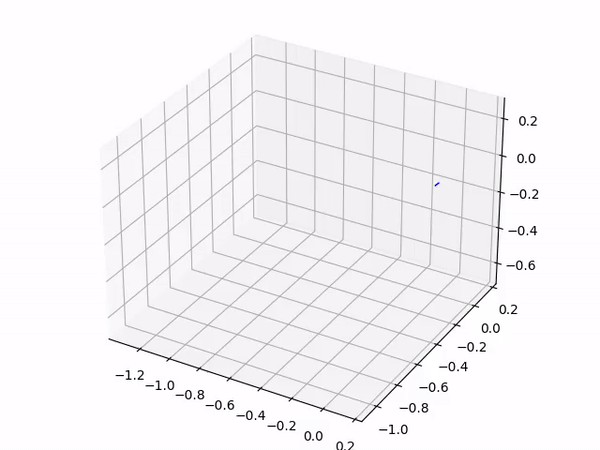
After a short delay you should see your gas molecule’s trajectory as it moves around the box! An interesting extension to this program is to add in more than 1 gas molecule; have a go and experiment!

Complete Brownian motion code

1
2
3
4
5
6
7
8
9
10
11
12
13
14
15
16
17
18
19
20
21
22
23
24
25
26
27
28
29
30
31
32
33
34
35
36
37
38
39
40
41
42
43
44
45
46
47
48
49

import numpy as np
import matplotlib.pyplot as plt
from matplotlib.animation import FuncAnimation
from IPython.display import HTML
import mpl_toolkits.mplot3d.axes3d as p3

fig = plt.figure()
ax = p3.Axes3D(fig)

N = 1000 # Number of points
T = 1.0
dt = T/(N-1)

dX = np.sqrt(dt) * np.random.randn(1, N)
X = np.cumsum(dX) # Cumulatively add these values to get the x positions of the particle

dY = np.sqrt(dt) * np.random.randn(1, N) 
Y = np.cumsum(dY) # Cumulatively add these values to get the y positions of the particle

dZ = np.sqrt(dt) * np.random.randn(1, N) 
Z = np.cumsum(dZ) # Cumulatively add these values to get the z positions of the particle

line, = ax.plot(X, Y, Z, color='blue', lw=1)

def animate(i):
    '''
    This function is iterated over by FuncAnimation to produce the frames necessary to produce the animation 
    
    Parameters:
    -----------
    i : int
        This is the index used to iterate through the coordinate arrays
    
    Returns:
    --------
    line : mpl_toolkits.mplot3d.art3d.Line3D
           This contains the line information which is updated each time the function is iterated over
    '''
    line.set_data(X[:i], Y[:i])
    line.set_3d_properties(Z[:i])

    return line

anim = FuncAnimation(fig, animate, interval=10, frames=N, repeat=False)

HTML(anim.to_html5_video()) # This is just for the Jupyter notebook which will not show the animation when using plt.show()

# if running locally, uncomment these two lines and remove the HTML command above.
#plt.show()

This produces the following output:

References

[1] Introduction to Probability Models 10th Edition, S. M. Ross, 2010, Elsevier, page 632.