T>T: Optimising Cumulative Sums in Python
The Problem:
We have a simple nested sum problem (aka cumulative sum): \[ \sum\limits_{a_i=0}^{a}\sum\limits_{b_i=0}^{b}\sum\limits_{c_i=0}^{c}\sum\limits_{d_i=0}^{d}\sum\limits_{e_i=0}^{e}\sum\limits_{f_i=0}^{f}\sum\limits_{g_i=0}^{a_i+b_i}\sum\limits_{h_i=0}^{c_i+d_i} \Omega, \] where \(\Omega\) represents arbitrary mathematical operations. There are 8 nested sums, with the inner two sums depending on the outer 4 sums. Let us put this into perspective:
For \(a = b = c = d = e = f = 10 \rightarrow\) 214358881 sum iterations
For \(a = b = c = d = e = f = 20 \rightarrow\) 37822859361 sum iterations
For \(a = b = c = d = e = f = 30 \rightarrow\) 852891037441 sum iterations
For \(a = b = c = d = e = f = 40 \rightarrow\) 7984925229121 sum iterations
For \(a = b = c = d = e = f = 50 \rightarrow\) 45767944570401 sum iterations
This just represents the number of ‘pass throughs’ of the sum that are required, and does not include the actual operations of the mathematics inside the nested sums. This is difficult from a computational standpoint due to the very large number of operations required. Let’s discuss how to implement this efficiently, and for this example, \(\Omega\) will have the form \[ \Omega = 2^{h_i - e_i + f_i - a_i - c_i - d_i + 1}(e_i^2 -2e_if_i - 7d_i)b_i!g_i!. \] A benchmark comparison of each solution is offered at the end of the post.
Solution 1: For Loops
The easiest option. Use for loops.
1
2
3
4
5
6
7
8
9
10
11
12
13
14
15
16
17
18
19
import numpy as np

def cumulative_sum_for_loops(a, b, c, d, e, f):
    '''
    This function calculates the cumulative sum using for loops
    '''
    Total = 0
    for ai in range(0, a):
        for bi in range(0, b):
            for ci in range(0, c):
                for di in range(0, d):
                    for ei in range(0, e):
                        for fi in range(0, f):
                            for gi in range(0, ai+bi)
                                for hi in range(0, ci+di)
                                    Total += (2)**(hi-ei+fi-ai-ci-di+1)*(ei**2-2*(ei*fi)-7*di)*np.math.factorial(bi)*np.math.factorial(gi)


    return Total
Pros: Very easy to program.
Cons: Very slow.
Solution 2: Cythonised For Loops
We will now use the same for loop structure but just use Cython to convert it into faster C code. The code below will be your .pyx file which you compile using a setup.py file.
1
2
3
4
5
6
7
8
9
10
11
12
13
14
15
16
17
18
19
20
21
22
23
24
25
26
27
28
import numpy as np

#cython: language_level=3
cimport cython
import numpy as np

@cython.boundscheck(False)  # Deactivate bounds checking
@cython.wraparound(False)   # Deactivate negative indexing.
cpdef cumulative_sum_for_loops(int a, int b, int c, int d, int e, int f):
    '''
    This function calculates the cumulative sum using for loops
    '''
    cdef int ai, bi, ci, di, fi, gi, hi
    cdef long double Total

    Total = 0
    for ai in range(0, a):
        for bi in range(0, b):
            for ci in range(0, c):
                for di in range(0, d):
                    for ei in range(0, e):
                        for fi in range(0, f):
                            for gi in range(0, ai+bi+1):
                                for hi in range(0, ci+di+1):
                                    Total += (2)**(hi-ei+fi-ai-ci-di+1)*(ei**2-2*(ei*fi)-7*di)*np.math.factorial(bi)*np.math.factorial(gi)


    return Total
Pros: Very easy to program.
Cons: Still slow.
Solution 3: Grid Evaluation
Grid evaluation involves constructing an n-dimensional grid, where each dimension represents the range of a single for loop. We can then sweep over this n-dimensional grid with the mathematics in \(\Omega\) and sum everything together in one go; effectively converting the problem to a much more efficient matrix problem.
1
2
3
4
5
6
7
8
9
10
11
12
13
14
15
import numpy as np
import scipy.special

def cumulative_sum_grid(a, b, c, d, e, f):
    '''
    This function calculates the cumulative sum using a grid
    '''
    # Setup the n-dimensional grid
    ai, bi, ci, di, ei, fi, gi, hi = np.ogrid[:a, :b, :c, :d, :e, :f, :a + b - 1, :c + d - 1]
    # Calculate the mathematics within the summations
    Total = (2.) ** (hi - ei - fi - ai - ci - di + 1) * (ei ** 2 - 2 * (ei * fi) - 7 * di) * scipy.special.factorial(bi) * scipy.special.factorial(gi)
    # Mask out of range elements for last two inner loops
    mask = (gi < ai + bi + 1) & (hi < ci + di + 1)

    return np.sum(Total * mask)
Pros: Very fast.
Cons: Very memory intensive.
This method is incredibly fast, but it uses a very large amount of Random Access Memory (RAM) to store the n-dimensional grid. My ThinkPad T430 has 16GB of RAM and the maximum value of \(a=b=c=d=e=f\) is 10 when the upper memory limit is reached. This method performs more computations than needed as the two inner loops have a varying number of iterations, hence will not require all the grid points allocated for it. This means you are evaluating more points on the grid than required and hence they are masked out at the end.
Solution 4: Grid Evaluation of Two Sums
Like Solution 2, but only evaluate the inner two sums using a grid.
1
2
3
4
5
6
7
8
9
10
11
12
13
14
15
16
17
18
def cumulative_sum_grid_two_sums(a, b, c, d, e, f):
    '''
    This function calculates the cumulative sum using a grid only on the inner two summations
    '''
    g = np.arange(a + b).reshape((-1, 1))
    h = np.arange(c + d)

    Total = 0
    for ai in range(0, a):
        for bi in range(0, b):
            gi = g[:ai + bi + 1]
            for ci in range(0, c):
                for di in range(0, d):
                    hi = h[:ci + di + 1]
                    for ei in range(0, e):
                        for fi in range(0, f):
                            Total += np.sum((2.) ** (hi - ei + fi - ai - ci - di + 1) * (ei ** 2 - 2 * (ei * fi) - 7 * di) * scipy.special.factorial(bi) * scipy.special.factorial(gi))
    return Total
Pros: Fast
Cons: Still heavy on memory for large values of \(a,b,c,d,e,f\) but better than solution 3. A good compromise.
Solution 5: JIT + Vectorisation
JIT stands for Just In Time compilation, which is a way of executing computer code involving compilation during execution of a program - at run time - rather than prior to execution. This is implemented via the Numba library.
Vectorisation is a very powerful programmatic technique well described by Wes McKinney:
“Arrays are important because they enable you to express batch operations on data without writing any for loops. This is usually called vectorization. Any arithmetic operations between equal-size arrays applies the operation elementwise.” - Wes McKinney
In this example, we are going to pre-evaluate some of the maths in \(\Omega\) and form a vector which we can index within the loops. The advantage of this is that for every for loop cycle the maths does not need to be reevaluated, instead being taken from the vector.
The maths in \(\Omega\) being vectorised is:
\[ \zeta = 2^{h_i - e_i + f_i - a_i - c_i - d_i + 1} \] Vectorising this expression means generating a vector containing all possible values the expression can equal. For us this means calculating the minimum and maximum value \(\zeta\) can be, providing us the two end points of our vector of pre-calculated results, which we can then fill.
Minimum value:
\(\zeta\) will be minimised when the exponent is as small as possible, i.e.
\[ \text{min}(h_i - e_i + f_i - a_i - c_i - d_i + 1) \] For addition operations we want to take the minimum value, and for subtraction operations we want to take the maximum value to form the smallest value possible. This means:
\(h_i = 0\) Smallest value \(h_i\) can be
\(e_i = e\) Largest value \(e_i\) can be
\(f_i = 0\) Smallest value \(f_i\) can be
\(a_i = a\) Largest value \(a_i\) can be
\(c_i = c\) Largest value \(c_i\) can be
\(d_i = d\) Largest value \(d_i\) can be
Resulting in:
\[ 0 - (e - 1) + 0 - (a - 1) - (c - 1) - (d - 1) + 1 = \mathbf{5 - (e + a + c + d)} \]
This represents the smallest value that \(\zeta\) can ever be; hence the smallest value in our vector.
Maximum value:
\(\zeta\) will be maximised when the exponent is as large as possible, i.e.
\[ \text{max}(h_i - e_i + f_i - a_i - c_i - d_i + 1) \] \(h_i = (c + d)\) Largest value \(h_i\) can be
\(e_i = 0\) Smallest value \(e_i\) can be
\(f_i = f\) Largest value \(f_i\) can be
\(a_i = 0\) Smallest value \(a_i\) can be
\(c_i = 0\) Smallest value \(c_i\) can be
\(d_i = 0\) Smallest value \(d_i\) can be
Resulting in:
\[ c + d + f + 1 \]
This represents the largest value that \(\zeta\) can ever be; hence the largest value in our vector. We will also precompute the two factorials, \(b_i!\) and \(g_i!\) which are much easier to vectorise.
Minimum value:
\(\text{min}(b_i!) = \text{min}(g_i!) = 0! = 1\)
Maximum value:
\(\text{max}(b_i!) = b!\)
\(\text{max}(g_i!) = (a + b)!\)
1
2
3
4
5
6
7
8
9
10
11
12
13
14
15
16
17
18
19
20
21
22
23
24
25
26
27
28
29
30
31
32
33
34
35
36
37
38
39
40
import numpy as np
from numba import njit # Import JIT library
from scipy.special import factorial # Import factorial function from scipy

def cumulative_sum_vectorised_math(a, b, c, d, e, f):
    '''
    This function vectorises the mathematical expression in the nested sums
    '''
    exp_min = 5 - (a + c + d + e) # Minimum value for exponent of zeta
    exp_max = c + d + f + 1 # Maximum value for exponent of zeta
    exp = 2. ** np.arange(exp_min, exp_max) # All possible values of zeta

    b_fac_grid = np.arange(e)
    g_fac_grid = np.arange(a + b)

    fact_b = factorial(b_fac_grid) # Factorial vector for b_i!
    fact_g = factorial(g_fac_grid) # Factorial vector for g_i!


    return cumulative_sum_JIT(a, b, c, d, e, f, exp_min, exp, fact_b, fact_g)

@njit()
def cumulative_sum_JIT(a, b, c, d, e, f, exp_min, exp, fact_b, fact_g):
    '''
    This function calculates the cumulative sum using JIT and vectorised maths
    '''
    Total = 0
    for ai in range(0, a):
        for bi in range(0, b):
            for ci in range(0, c):
                for di in range(0, d):
                    for ei in range(0, e):
                        for fi in range(0, f):
                            for gi in range(0, ai + bi + 1):
                                for hi in range(0, ci + di + 1):
                                    # We now index from the vectors, exp_min, exp_max, fact_b and fact_g whilst also applying JIT compilation using @njit()
                                    Total += exp[hi - ei + fi - ai - ci - di + 1 - exp_min] * (ei * ei - 2 * (ei * fi) - 7 * di) * fact_b[bi] * fact_g[gi]

    return Total
Pros: Fast and not RAM intensive.
Cons: Vectorisation may prove much more difficult for more complex examples, and JIT compilation in python does not work well with NumPy or SciPy. This is one of the main reasons why \(b_i!\) and \(g_i!\) were precomputed as JIT will not work with the factorial implementation of SciPy. This is also limited to machine double precision which will be important later.
Benchmark
The following benchmark was conducted on my ThinkPad T430 laptop: Intel i7-3520M CPU @ 2.90GHz × 4, 16GiB RAM. For the purposes of this benchmark, \(a=b=c=d=e=f\) to simulate the toughest problem.
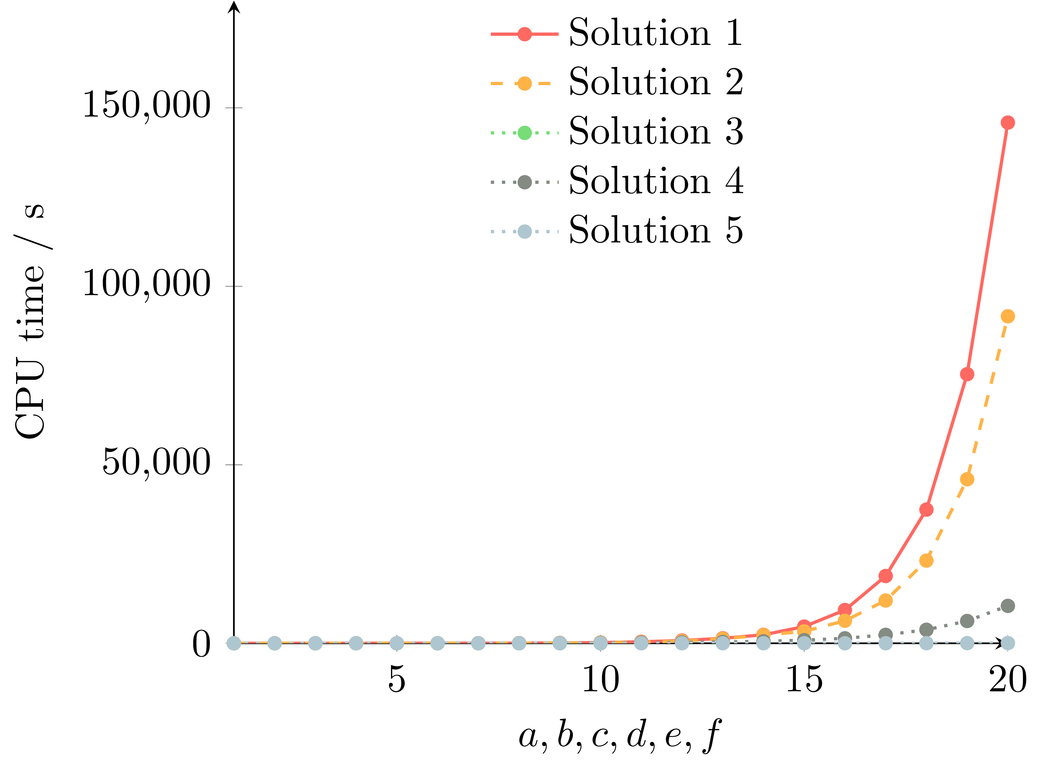
Solution 3 is plotted, however I could only calculate up to \(a=b=c=d=e=f=10\) before my RAM limit was reached, so its data points are hidden behind the others.
As the above plot highlights, for loops are embarrasingly slow for this type of cumulative sum problem. Solution 2 used Cython and achieved a nice speedup. Solution 3 used grid evaluation which was fast but uses too much memory for conventional hardware. Solution 4 only used grid evaluation for the inner two summations and results in a substantial speedup over the Cythonised for loops. However, Solution 5 is the clear winner which used a combination of JIT and vectorised mathematics. It is over 3000 times faster than the for loop implementation for \(a=b=c=d=e=f=20\).
Solution 1: 145873.077 s
Solution 5: 48.441 s
Conclusion
This post has shown how to optimise a cumulative sum problem in Python. Five solutions were presented, and it was shown how a combination of JIT and vectorised mathematics resulted in an over 3000 x speedup over conventional for loops.
The inspiration behind this post comes from a mathematical calculation in my research which required a nested summation similar to this problem, but evaluated over 200,000 times for different values of \(a, b, c, d, e, f\). Not only this but it also required 200-digit precision, adding an even greater complexity to the problem.
The precision of this calculation is not discussed here, but going to high enough values of \(a,b,c,d,e,f\) will result in severe accumulation of errors due to the limitation of hardware double precision. Another post will discuss how to handle this.
The techniques discussed here are quite general, so can hopefully find place in any problems where it is tempting to default to nested for loops. parallelisation was also not discussed as we know ahead of time how much faster it will be (usually no. cores - 1 speedup).