T>T: FROST III, the Hartree–Fock Limit in Milliseconds

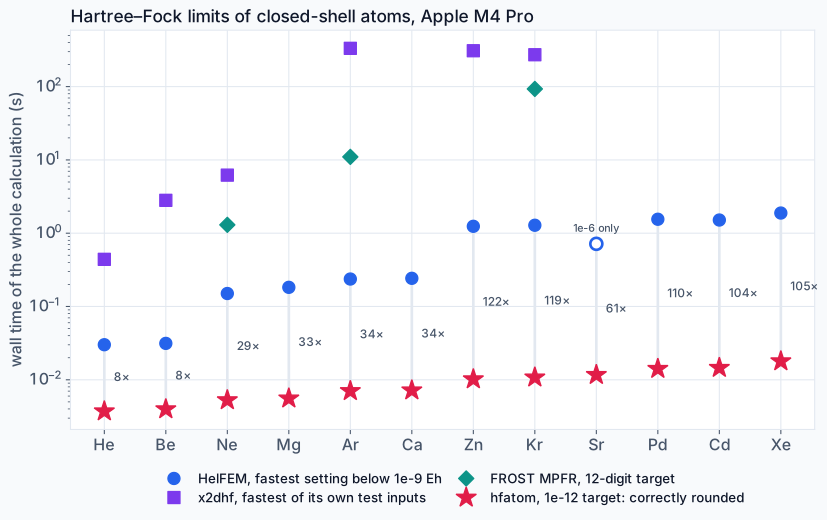
TLDR: In this post learn how to turn FROST, which certifies Hartree–Fock energies to hundreds of digits in hours, into hfatom, a 675-line C program (with Python bindings) that gets the Hartree–Fock limit of any closed-shell atom in double precision in milliseconds. For all fourteen atoms and ions with a certified limit, from H⁻ to xenon, the energy it returns is that limit correctly rounded, the nearest double, in 0.6 ms (helium) to 12.6 ms (xenon). Against HelFEM at its best settings, chosen with hindsight from 3204 runs, it is 7 to 380 times faster; Gaussian basis sets never get closer than \(10^{-4}\) hartree, and x2dhf takes seconds to minutes. The method is a Lagrange mesh and Newton’s method, and the precision comes from one rule: rounding errors in the numbers that define the problem go straight into the energy, while errors in the solution barely touch it, so only the first kind is computed exactly.

This post is part of a series on Hartree-Fock theory:

• Restricted Hartree-Fock in 100 Lines: The original post; start here if new to HF
• Unrestricted Hartree-Fock in 100 Lines: Open shells and spin contamination
• The Integrals at the Heart of Hartree-Fock Theory: Every integral the basis-set approach needs, derived from scratch
• Hartree–Fock to 500 Significant Figures with FROST: We throw the basis set away, for helium and beryllium
• FROST II, Certified Hartree–Fock from Neon to Xenon: \(p\) and \(d\) shells, and 104 certified figures for xenon
• FROST Fast, the Hartree–Fock Limit in Milliseconds: You are here, and we trade digits for speed

The result

Since the last post the Hartree–Fock limit of xenon is known to 104 significant figures. A double-precision number holds about 16 of them, and blue below are the figures that the certified value and the nearest double share. hfatom returns exactly that double, with an error of 0.16 of the spacing between neighbouring doubles, and it takes 12.6 ms to do so on my laptop.

Xenon, certified (FROST II, 104 significant figures)

−7232.1383638718408882092892165590604072114337605157184882466310507041952021682604466883605882653741993730

Xenon, hfatom in double precision (12.6 ms), the double written out exactly: it prints as −7232.138363871841, and no double is closer

−7232.1383638718407382839359343051910400390625

The same is true of all fourteen atoms and ions with a certified limit, from H⁻ to xenon (Part IV has them all). For comparison, here is xenon with the other ways of getting a Hartree–Fock limit, all on the same machine:

method (xenon)	error (Eh)	wall time
Gaussian basis, uncontracted ANO-RCC, 206 functions (PySCF)	\(6.3\times10^{-3}\)	9.2 s
HelFEM, its fastest setting below \(10^{-9}\) Eh	\(1.8\times10^{-11}\)	1.88 s
HelFEM, the most accurate of 182 settings	\(4.4\times10^{-12}\)	2.54 s
hfatom (whole process, including start-up)	\(1.5\times10^{-13}\)	17.9 ms

Wall time of the whole calculation for twelve closed-shell atoms. hfatom (red stars) is asked for \(10^{-12}\) Eh and returns the correctly rounded limit; HelFEM (blue) is given its fastest setting below the easier target of \(10^{-9}\) Eh, picked from 3204 runs with the answer known in advance; for strontium no setting got there, and the hollow circle is its time for \(10^{-6}\). The numbers are the ratios between the two. x2dhf (purple) is the fastest of its own test inputs for each atom, and FROST in MPFR (teal) the 12-digit run.

Introduction, or what do you do with 500 digits?

The first two FROST posts were about digits, and I am still very fond of the 504 figures of neon, but nobody needs them to compute anything. What people actually do with Hartree–Fock limits is compare against them: the error of a basis set is measured from the limit, a new density functional code checks its exchange against it, and a correlation energy is defined as the distance below it. For all of that, double precision is plenty, and what matters is that the number is right to the last digit and that it arrives quickly enough to be called inside a loop.

So the question for this post is simple to state. If you only want 16 digits, how fast can you get them, and can the ideas from FROST make that faster than anything that already exists? The goal I set myself was the fastest version that is physically possible on a laptop, which is a nice thing to aim for even if it cannot be proved.

The competition is good, and it has a long history. Nearly all of quantum chemistry uses Gaussian basis sets, which are fast but converge slowly towards the limit, so even the largest standard sets stop about \(10^{-4}\) hartree short of it. The limit itself is the business of fully numerical methods, which go back to Hartree and were made routine for atoms by Charlotte Froese Fischer’s finite-difference programs; since then atomic limits have been computed with Slater-type expansions (Clementi and Roetti), B-splines (Saito) and finite elements, and Susi Lehtola’s 2019 review is the place to start if you want the whole story. Three of these methods matter most for this post:

• x2dhf, by Jacek Kobus and now Susi Lehtola, solves the equations by high-order finite differences on a two-dimensional grid and has been the reference for diatomic molecules for decades; it does atoms too
• HelFEM, by Susi Lehtola, uses finite elements and is the fastest atomic code I could run: it reaches \(10^{-12}\) hartree for neon in under 0.3 s
• Cinal’s pseudospectral method (2020) is the closest in spirit to this post. It represents each orbital by its values at Legendre–Lobatto points mapped onto the whole half-line, gets 14 significant figures in double precision from only 33 to 71 points, and gets 25 in quadruple precision, which was the record from calcium to xenon until FROST II. His program is not in the race below, so the fairest comparison is his own report: under 3 s of CPU time for 100 points and 200 iterations on a 2011 laptop, with energies two or three figures short of a double

FROST itself, run at 12 digits in MPFR, takes 1.3 s for neon and 93 s for krypton, which is perfectly fine for setting records.

I kept the scope tight: closed-shell atoms first, with diatomics later (Part VI has a preview). “Faster” means the wall time to get within \(10^{-6}\), \(10^{-9}\) and \(10^{-12}\) hartree of the true limit, with every code at its best settings (that I could find anyway) on the same machine.

Try the code yourself

The code lives in the FROST repository, github.com/adambaskerville/frost, in the fast/ folder. The benchmark scripts, the raw timings of every run in this post and the figure script are in FROSTFastCode/, next to this post.

file	what it does
fast/hfatom.c	the solver, one C file of 675 lines
fast/frostfast.py	Python bindings through ctypes, compiled on first use
fast/test_hfatom.py	checks all fourteen certified limits (about 0.2 s)
FROSTFastCode/bench_atoms.py	the HelFEM settings scan and the timing runs
FROSTFastCode/bench_other.py	Gaussian basis sets (PySCF) and x2dhf

You need a Mac with a C compiler, since the linear algebra comes from Apple’s Accelerate framework, and Python 3 for the bindings and the test, which use only the standard library. I will probably get around to writing a generic version of this for Linux too (or just throw it at your AI of choice to do).

git clone https://github.com/adambaskerville/frost && cd frost/fast
cc -O3 -mcpu=native -o hfatom hfatom.c -framework Accelerate

./hfatom Xe                                    # neutral ground state, target 1e-12
./hfatom 54 "1s 2s 2p 3s 3p 3d 4s 4p 4d 5s 5p" --tol 1e-9
./hfatom 1 1s -v                               # H-, and the grid it chose
python3 test_hfatom.py                         # all fourteen certified limits

The first command prints the energy, the virial ratio and the orbital energies:

Xe  Z=54  1s 2s 2p 3s 3p 3d 4s 4p 4d 5s 5p
E      = -7232.1383638718407
virial = -1.910e-14  (-V/T - 2)
eps 1s  = -1224.3977774585344
eps 2s  = -189.3401229314705
...
eps 5p  = -0.4572900578519
time   = 12.68 ms

From Python the same solver is one function call, and without the cost of starting a process a hundred neon atoms take 0.2 s:

import frostfast

r = frostfast.atom("Kr")      # or atom(36), atom(36, "1s 2s 2p 3s 3p 3d 4s 4p", tol=1e-9)
r["E"], r["eps"]["4p"]        # -2752.0549773455764, -0.5241866810268421
r["N"], r["seconds"]          # 63 nodes, 0.0062 s

Birds-eye view

1. Part I is the race: what “faster” means, and how every competitor was given its best chance
2. Part II is the method: a Lagrange mesh, a variational functional and Newton’s method
3. Part III is where double precision goes to die, and the rule that keeps every digit
4. Part IV is the results, with every method on one plot
5. Part V is the list of things that I broke along the way, and Part VI the lessons and what comes next

Part I: The rules of the race

A benchmark is only as honest as its rules, so here they are before any numbers.

• The truth is known. Every error in this post is measured against the certified limits of the FROST papers, which have at least 100 significant figures for every atom here; the only exceptions are four atoms beyond xenon in Part IV, which are measured against Cinal’s 25-figure energies. No code is judged against itself, against an extrapolation, or against another code
• Three targets. For each atom, the wall time to get within \(10^{-6}\), \(10^{-9}\) and \(10^{-12}\) hartree of the limit. The last one is close to the spacing between doubles for the heavy atoms (xenon’s is \(9.1\times10^{-13}\)), so it is a test of whether a code keeps every digit
• One machine. Everything ran on the 12 cores of an Apple M4 Pro laptop, one job at a time with nothing else running, and the times are medians of repeated runs of the whole process, start-up included
• Best settings, chosen with hindsight. HelFEM has four knobs that decide its accuracy: the primitive polynomial basis, the number of nodes per element, the number of elements and the practical infinity \(R_\max\). I scanned all of them, 3204 runs in total, and for each atom and target took the fastest run whose true error was below the target. In real life nobody can make that choice without knowing the answer, so this is generous to HelFEM. hfatom gets no such help; it is only told the target with --tol
• Everyone else at their best too. x2dhf is the OpenMP build, run on the test inputs that its authors ship for each atom, and timed by its own clock summed over the stages of each input, which leaves out its driver script. The Gaussian basis sets are PySCF’s RHF with the largest standard basis sets, timed for the integrals and the SCF alone, without the Python start-up or building the molecule

Two of the codes needed help to build on a Mac, neither of which touches the numerics. HelFEM uses the special functions std::cyl_bessel_i and std::sph_legendre, which Apple’s C++ library does not provide, so I added small replacements. x2dhf builds with the current gfortran, but its run-time library then rejects one of x2dhf’s old-style FORMAT statements, and I rebuilt it with -std=legacy (more on how I found that in Part V).

Part II: The method

1. Why not just FROST in double precision?

FROST integrates the radial equations outwards as Taylor series and shoots. In FROST II the krypton \(1s\) orbital wanted to grow by a factor of \(10^{1701}\) over the range, and multiple shooting dealt with that by spending more digits and more segments. In double precision there are only 16 digits to spend, so the segments would have to be short and many, and every step would still cost a Cauchy product. I engineered FROST’s machinery for precision, not speed.

For double precision the better tool is a global spectral method whre each orbital is represented by its values at a few dozen well-chosen points, the error falls exponentially with the number of points, and the whole problem becomes dense linear algebra on matrices of a few hundred rows, which is exactly what a laptop’s matrix hardware is best at. What carries over from FROST is everything that is not about arithmetic: Hartree’s radial equations rather than a basis expansion, one common wall for all orbitals, Newton’s method, and the habit of checking every digit against something certified.

Spectral grids for atomic Hartree–Fock are not new. Godefroid, Liévin and Heenen used a Lagrange mesh for two-electron atoms in 1989, and Cinal’s pseudospectral method solves the closed-shell equations from helium to nobelium on a grid of the same family. What this post adds is in how the grid is used: an energy that is variational rather than collocated (§7), Newton’s method in place of a fixed-point iteration (§5), and a final energy evaluated exactly where it matters (§8–9), which together turn 14 figures into the correctly rounded double.

2. A Lagrange mesh

The orbitals are written as \(P_a(r) = rR_a(r)\), and the radial coordinate is mapped to \(t\in(0,2]\) by

\[r = a\left(e^{St/2}-1\right),\qquad S = \ln(1+R/a),\]

so that \(t = 2\) is the wall at \(r = R\) and the nodes crowd towards the nucleus, where every orbital has its cusp. Each orbital is represented by its values at the \(N\) right Gauss–Radau nodes \(t_j\), which include the wall and exclude the origin, through the Lagrange functions \(\ell_j(t)\) that equal one at \(t_j\) and zero at the other nodes. Multiplying by \(t/t_j\) gives the regularised Lagrange functions of Baye, which vanish at \(r = 0\), so the boundary condition at the nucleus is built in rather than imposed.

The trick that makes this a Lagrange mesh is that every integral is done by the same Gauss–Radau quadrature, at the same nodes. The overlap of two basis functions is then zero unless they belong to the same node, so the mass matrix is diagonal, and the energy becomes a polynomial in the nodal values \(P_a(r_i)\):

\[E[P] = \sum_a w_a\sum_i W_i\Big[\frac{l_a(l_a+1)}{2r_i^2}-\frac{Z}{r_i}\Big]P_a(r_i)^2 + \sum_a \frac{w_a}{2}\sum_m\frac{w_m}{r'_m}\Big(\frac{dP_a}{dt}\Big)_m^2 + E_J - E_K,\]

where \(W_i = w_ir'(t_i)\) are the quadrature weights in \(r\), \(w_a = 2(2l_a+1)\) is the occupation, and the derivative \(dP/dt\) at the nodes is a matrix \(D\) applied to the nodal values. The Coulomb and exchange energies \(E_J\) and \(E_K\) need the multipole potentials, which come next.

One choice from the original FROST did not survive as FROST works with Hartree’s \(f = P/r^{l+1}\), which keeps every Taylor coefficient polynomial and made the certificate possible. On a global mesh it is a disaster for \(l\ge1\), because the weights \(r^{2l+2}\) in the energy then span 38 orders of magnitude for an \(f\) shell, which double precision cannot hold, and the lowest eigenvalues are destroyed.

3. The potentials on the same mesh

Exchange between orbitals \(a\) and \(b\) needs the potential of the density \(P_aP_b\) for every multipole \(k\). Writing it as \(Y^k(r)/r\), as in FROST, \(Y^k\) solves

\[\frac{d^2Y^k}{dr^2} - \frac{k(k+1)}{r^2}Y^k = -(2k+1)\frac{P_aP_b}{r},\qquad Y^k(0) = 0,\qquad RY^{k\prime}(R)+kY^k(R) = 0,\]

where the condition at the wall is the exact one: outside the wall the density is zero and the solution is \(r^{-k}\). On the mesh this is a symmetric positive-definite system \(K_kY = (2k+1)\,v\odot P_aP_b\) with \(v_i = W_i/r_i\), the discrete Galerkin version of the equation, and since the mesh is fixed its inverse \(G_k = (2k+1)K_k^{-1}\) is computed once, by a Cholesky factorisation, before the iterations start. Each Coulomb or exchange integral is then a quadratic form \(B_k(\rho,\rho) = \rho^{\mathsf T}G_k\rho\) in the density sampled at the nodes, and the whole energy is a polynomial of degree four in the nodal values.

4. One wall, again

FROST II needed one common wall for all orbitals, because the multipoles hand every orbital the tail of the outermost one. Here one wall comes for free, since every orbital lives on the same mesh, and it brings the same reward. The canonical orbitals of each angular momentum are eigenvectors of one Fock matrix, so they are orthogonal without any constraint, and the off-diagonal Lagrange multipliers that made the first FROST post so painful never appear.

5. Newton’s method, all the way down

The standard way to solve the Hartree–Fock equations is the self-consistent field iteration with DIIS: build the Fock matrix from the current orbitals, diagonalise it, mix, repeat. It is robust, but it converges linearly, and the last few digits of a heavy atom cost as many iterations as the first few. Second-order methods that converge quadratically have been around in basis-set codes since Bacskay’s QC-SCF of 1981, and hfatom uses the SCF iteration only to get started:

1. A guess from Thomas–Fermi. The orbitals start as eigenvectors of a screened Thomas–Fermi potential (Tietz’s analytic form, with Latter’s \(-1/r\) tail), which is already a fair picture of where the shells are
2. A few SCF steps. SCF with DIIS runs until the commutator of the Fock and density matrices is below \(10^{-6}\), which takes eight iterations for xenon. That is far from converged, but it is inside Newton’s basin

3. Two Newton steps. Newton’s method on the Lagrangian $$L = E - \sum_a w_a\varepsilon_a(\langle a

   a\rangle-1)\(solves for every nodal value of every orbital and every orbital energy at once, with the exact Hessian assembled analytically, including the response of every Coulomb and exchange potential through the\)G_k\(. Scaling the orbital rows by\)2l_a+1\(and the norm rows by\)-(2l_a+1)$$ makes the matrix symmetric. For xenon it has 737 rows (11 orbitals at 66 inner nodes, plus 11 orbital energies), one dense LU factorisation per step

Newton converges quadratically, so from an SCF error of \(10^{-6}\) the first step should land near \(10^{-12}\) and the second at the floor of double precision. Two steps is not a tolerance I tuned for speed; one step left zinc two units in the last place off, and the second removed them.

6. The code chooses its own grid, and keeps a canary

hfatom has no settings to tune, which in a benchmark against an oracle-tuned competitor is the point. The scale is \(a = 3/Z\), which puts the innermost nodes inside the \(1s\) shell for every atom, and the number of nodes for a target of \(10^{-d}\) hartree is

\[N = \lceil 10\ln Z + 2d + 3\rceil,\]

plus \((Z-54)/2.5\) beyond xenon. I calibrated this rule on the certified limits from helium to xenon, and it gives 67 nodes for xenon at \(10^{-12}\). The wall starts at \(R = 40\) bohr and moves out when the decay of the outermost orbital requires it. The energy error caused by a wall falls like \(e^{-2\kappa R}\) with \(\kappa = \sqrt{-2\varepsilon_\text{HOMO}}\), and a fit to FROST’s wall studies gives \(E_R - E_\text{HF}\approx3\times10^4e^{-2\kappa R}\), so the wall is moved until that is below the target. Only H⁻, whose outermost electron is barely bound, needs more than 40 bohr: it moves to 63.

An under-resolved spectral grid does not fail gracefully. Mercury at 71 nodes converged happily to a wrong solution, with an energy that looked plausible at a glance. What gave it away was the virial theorem: for the exact Hartree–Fock solution \(-V/T = 2\), a resolved grid gives $$

{-V/T}-2

\approx10^{-14}\(, and mercury's wrong solution had\)10^{-4}\(. So the virial ratio is the canary, as it is in Cinal's work, where it is the measure of how well a grid has converged. If it is off by more than\)10^{-9}$$, hfatom enlarges the grid by 15% and solves again, and that is why the grid rule now has its extra term beyond xenon.

Part III: Where double precision goes to die

My first versions of this method got neon to about \(10^{-9}\) hartree. Getting the remaining digits took most of the work, and almost every lost digit was lost the same way, which is the most useful thing in this post if you ever do floating-point work on a variational problem.

The reason is a fact every quantum chemist knows in another form. At a stationary point of a functional, an error \(\delta\) in the orbitals changes the energy only by \(O(\delta^2)\), which is why variational energies are so much more accurate than the wavefunctions they come from. But an error in the functional itself, in the numbers that define what is being minimised, changes the energy by \(O(\delta)\). In double precision every number carries a relative rounding error of about \(10^{-16}\), and the heavy atoms have energy terms of \(10^4\) hartree, so any number that enters at first order costs \(10^{-12}\). Every lesson in this part is an instance of one rule: find the numbers that enter at first order, and only compute those exactly.

7. Make the energy stationary

My first version used collocation, which asks the equations to hold exactly at the nodes. It is the textbook way to use a Lagrange mesh and it converges nicely, but the energy it produces is not stationary in anything, so noise in the orbitals enters it at first order. Adding \(10^{-10}\) of random noise to the neon orbitals moved the energy by \(10^{-9}\). The Galerkin version of §2, which minimises a discrete energy functional, has the same mesh and the same cost, but its energy is stationary, so the same noise moves it only by something of the order of the noise squared, and the rounding noise in the orbitals stops mattering at all. Cinal’s pseudospectral method is also a collocation method, and his double-precision energies show the symptom you would expect: they wobble in the last figures from one iteration to the next, and he reaches 15 figures by averaging the energy over a hundred iterations.

8. Round nothing that defines the functional

With a stationary energy, the next floor came from the functional itself. The differentiation matrix \(D\), the nodes, the quadrature weights and the mapped mesh \(r_i\), \(W_i\) and \(v_i\) all define \(E[P]\), and rounding any of them perturbs the functional at first order:

• The kinetic matrix. Forming \(D^{\mathsf T}\text{diag}(w/r')D\) in double precision put neon \(5\times10^{-11}\) hartree off
• The nodes. numpy’s Gauss–Legendre roots, a natural starting point, are off by up to \(10^{-14}\) near the ends of the interval, which gave weight errors of \(10^{-12}\). hfatom solves for the Radau nodes by Newton’s method, with the last step in double-double
• The mesh. With \(D\) and the nodes exact, xenon’s energy still scattered by up to five units in the last place as the grid changed, from the weights and mapped nodes computed in plain double

Computing everything in higher precision would fix this and make every iteration several times slower. It is also unnecessary, because the solver does not need exact operators. Newton’s method on a functional perturbed by \(10^{-16}\) converges to orbitals that are \(O(10^{-16})\) away from the stationary point of the exact functional, and those orbitals enter the exact energy only at second order. So hfatom does all the work in plain double precision, and evaluates the final energy once, at the end, with exact operators: the nodes, weights, mesh and \(D\) in double-double (two doubles per number, about 32 digits), and every product formed exactly with fused multiply-adds, using the error-free transformations of Ogita, Rump and Oishi. It is the same idea as the cheap Jacobians of FROST II, where the accuracy came from the residual and not from the Jacobian.

The Coulomb and exchange integrals need one more step, because they involve \(G_k = (2k+1)K_k^{-1}\), and inverting \(K_k\) in double-double would be expensive. Instead each integral is evaluated in the variational form

\[B_k(\rho,\rho) = 2\rho^{\mathsf T}Y - \frac{Y^{\mathsf T}K_kY}{2k+1},\qquad Y = G_k\rho,\]

which equals \(\rho^{\mathsf T}G_k\rho\) when \(Y\) is exact and is stationary in \(Y\). So \(Y\) can come from the double-precision \(G_k\), and only the explicit \(K_k\), which is cheap to apply in double-double, needs to be exact. This is the trick behind Dunlap’s robust fitting of Coulomb integrals in density functional codes, where the error being made second order is that of an auxiliary basis; here it is rounding. The Coulomb term also needs a single potential for the total density, rather than a sum of orbital-pair potentials, or the rounding of each pair adds up.

9. Orthonormality is part of the functional

The energy expression assumes orthonormal orbitals, and a Newton step meets the constraints only to first order. It leaves norm errors and same-\(l\) overlaps of the order of the step squared, which enter the energy at first order through the orbital energies, and xenon’s \(1s\) has \(\varepsilon = -1224\) hartree. Stopping Newton a little early left energies \(10^{-12}\) to \(10^{-10}\) below the limit. Löwdin orthonormalisation of each \(l\) block before the energy is evaluated removes the defects, but only to rounding, and for xenon’s \(1s\) pair a norm defect of \(10^{-16}\) times 1224 hartree is already a quarter of a unit in the last place. So the final energy also carries the first-order correction

\[\Delta E = -\sum_a w_a\varepsilon_a\big(\langle a|a\rangle-1\big),\]

with the norms computed in double-double. Off-diagonal overlaps need no correction, because for canonical orbitals the off-diagonal multipliers are zero, so they enter at second order.

10. What the rule buys

Here is xenon before and after the last part of the rule, the double-double mesh and the norm correction, as the grid changes (errors in units of the spacing between doubles at 7232, \(9.1\times10^{-13}\) hartree):

grid	mesh in double	mesh exact, norms corrected
67 nodes, wall at 40 bohr (the default)	−2.84	+0.16
67 nodes, 50 bohr	−0.84	+0.16
80 nodes, 40 bohr	−4.84	+0.16
90 nodes, 50 bohr	+0.16	+0.16
100 nodes, 50 bohr	+1.16	+0.16

Before, the energy landed on any of seven neighbouring doubles depending on the grid, and on the right one only by luck. After, it does not move at all, because what is left is the discretisation and wall error of the grid, which is far below a unit in the last place. The exact energy costs 0.67 ms, about 5% of xenon’s time (Part IV has the full breakdown).

Lesson. In double precision the digits are almost never lost in the hard part of the calculation. They are lost in the bookkeeping: a weight computed in double, a product rounded before it is summed, a matrix formed once and trusted forever.

For a variational problem, sort every number into one of two piles: the ones you solve for, which enter the energy squared, and the ones that define what you are solving, which enter it linearly. Do the first pile as cheaply as you like and the second pile exactly, once, at the end.

Part IV: Results

Every certified atom, correctly rounded

These are the energies hfatom returns with its default target, against the certified limits. The last column is the time of the calculation inside the library; starting a process adds 3 to 5 ms on top.

atom	E (hfatom)	error (Eh)	units in the last place	time
H⁻	−0.48792973437085174	\(+6.7\times10^{-18}\)	+0.12	1.4 ms
He	−2.861679995612239	\(-7.9\times10^{-17}\)	−0.18	0.6 ms
Li⁺	−7.236415201452256	\(+4.4\times10^{-16}\)	+0.50	0.6 ms
Be	−14.5730231683164	\(-4.1\times10^{-16}\)	−0.23	1.0 ms
Ne	−128.54709810938203	\(+8.2\times10^{-15}\)	+0.29	2.1 ms
Mg	−199.6146364245067	\(+1.1\times10^{-14}\)	+0.40	2.5 ms
Ar	−526.8175128027234	\(-4.5\times10^{-14}\)	−0.39	3.2 ms
Ca	−676.7581859245134	\(+1.4\times10^{-14}\)	+0.12	4.5 ms
Zn	−1777.848116191361	\(+8.3\times10^{-14}\)	+0.37	6.2 ms
Kr	−2752.0549773455764	\(+6.5\times10^{-14}\)	+0.14	6.7 ms
Sr	−3131.5456864385574	\(-1.8\times10^{-13}\)	−0.40	7.5 ms
Pd	−4937.921024070101	\(+2.3\times10^{-13}\)	+0.26	10.1 ms
Cd	−5465.133142530087	\(-4.1\times10^{-13}\)	−0.45	10.4 ms
Xe	−7232.138363871841	\(+1.5\times10^{-13}\)	+0.16	12.6 ms

Every error is below half a unit in the last place, which is the definition of correct rounding: no double is closer to the true limit. Lithium’s +0.50 looks like a coin toss, and it nearly is, because its certified limit happens to lie almost exactly halfway between two doubles; hfatom returns the nearer one. The test script checks exactly this, that each energy is the double nearest to the certified value, so it fails if a single bit changes.

Beyond xenon there are no certified limits, but Cinal’s quadruple-precision energies have 25 figures, and from neon to xenon every one of them agrees with the certified limits. Against them, hfatom’s energies of barium, ytterbium, mercury and radon are correctly rounded too, with errors of +0.20, +0.34, −0.26 and +0.38 units in the last place, in 15 to 44 ms.

Against HelFEM

Here is the race of Part I, with HelFEM at its oracle-chosen best for each target and hfatom told only the target. Both times are for the whole process, start-up included, as medians of repeated runs (2 for HelFEM, 11 for hfatom).

Each cell is HelFEM’s time, hfatom’s time and the ratio between them.

atom	\(10^{-6}\) Eh	\(10^{-9}\) Eh	\(10^{-12}\) Eh
He	0.04 s / 3.5 ms (12×)	0.03 s / 3.6 ms (8×)	0.04 s / 3.7 ms (9×)
Be	0.03 s / 3.8 ms (7×)	0.03 s / 4.0 ms (8×)	not reached / 4.0 ms
Ne	0.11 s / 4.6 ms (24×)	0.15 s / 4.9 ms (30×)	0.29 s / 5.3 ms (54×)
Mg	0.11 s / 4.8 ms (22×)	0.18 s / 5.5 ms (33×)	not reached / 5.6 ms
Ar	0.16 s / 5.8 ms (28×)	0.24 s / 6.2 ms (38×)	0.31 s / 7.0 ms (45×)
Ca	0.16 s / 6.2 ms (26×)	0.24 s / 6.8 ms (36×)	not reached / 7.2 ms
Zn	0.78 s / 7.4 ms (105×)	1.24 s / 8.3 ms (150×)	not reached / 10.2 ms
Kr	0.77 s / 8.0 ms (96×)	1.28 s / 9.3 ms (138×)	1.79 s / 10.8 ms (167×)
Sr	0.72 s / 10.5 ms (68×)	not reached / 10.9 ms	not reached / 11.7 ms
Pd	0.91 s / 10.7 ms (84×)	1.55 s / 11.8 ms (131×)	5.38 s / 14.1 ms (381×)
Cd	1.05 s / 11.6 ms (91×)	1.51 s / 12.0 ms (126×)	not reached / 14.6 ms
Xe	1.01 s / 12.9 ms (78×)	1.88 s / 14.9 ms (126×)	not reached / 17.9 ms

hfatom met every target for every atom; its errors, and HelFEM’s settings and errors, are in FROSTFastCode/data/bench_atoms.md.

Three things stand out. The speed-up grows with the atom, from 7 to 12 for helium and beryllium, where both codes spend most of their time starting up, to between 60 and 380 from zinc onwards. HelFEM’s default basis (--primbas=5, Hermite interpolating polynomials) is about five times slower than the settings in the table, and lands \(10^{-10}\) below the limit, so the default is not what you want either. And at \(10^{-12}\) HelFEM runs out of digits: for seven of the twelve atoms, none of the 3204 settings got within \(10^{-12}\), and the closest it gets to xenon is \(4.4\times10^{-12}\). That is the same floor that hfatom had before §8 and §9, which suggests, though I have not checked, that HelFEM’s last digits go the same way.

Every method on one plot

The table compares two codes at three targets. The plot below puts every method on the same axes for neon and krypton, with every HelFEM run from the scan, so you can see the whole trade-off between time and accuracy.

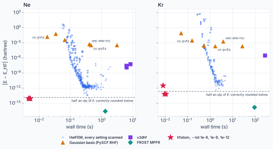Error against wall time for neon and krypton, both axes logarithmic. Pale blue dots are all of HelFEM’s settings from the scan, orange triangles Gaussian basis sets in PySCF, purple squares x2dhf on its own test inputs, the teal diamond FROST in MPFR at 12 digits, and the red stars hfatom at its three targets. The dashed line is half a unit in the last place of \(E\), so an energy below it is correctly rounded.

• Gaussian basis sets are fast and stop early. The correlation-consistent sets cc-pVDZ to cc-pV5Z bring neon from \(6\times10^{-2}\) to \(3.3\times10^{-4}\) hartree in 0.02 to 0.45 s, the core–valence cc-pCV5Z costs seven times as much for no gain, and the uncontracted ANO-RCC set, with 100 functions, stops at \(5\times10^{-4}\). This floor is the basis set, not the code: Gaussians have no cusp at the nucleus and decay too fast, so the last digits need ever more functions. (The contracted ANO-RCC sets are built for relativistic Hamiltonians, and in non-relativistic Hartree–Fock they are 0.5 hartree off for argon and 25 for krypton, so they are not plotted.)
• x2dhf is accurate but slow for atoms, which is not what it was built for: it solves a two-dimensional problem in prolate spheroidal coordinates even when one dimension would do. Its own inputs take 0.44 s for helium (\(1.1\times10^{-10}\)), 6 to 8 s for neon (\(1\) to \(6\times10^{-8}\)), 333 s for argon (\(10^{-8}\)), and 272 s for krypton and 309 s for zinc, which stop \(3\times10^{-6}\) and \(6\times10^{-6}\) from the limit. Its most accurate krypton input, according to the reference output shipped with it, runs for 4.1 hours on 20 cores
• FROST in MPFR at 12 digits takes 1.3 s for neon and 93 s for krypton, and its strength is elsewhere: it is the only code here whose answer comes with a certificate
• hfatom sits in the bottom-left corner, alone: about 5 ms for neon and 8 to 11 ms for krypton as whole processes (2 and 7 ms inside the library), and at its tightest target nothing between it and the true limit but the rounding to a double

Where the time goes

Inside the library call, the time divides up as follows (medians of a separate set of 25 runs, so the totals differ slightly from the table above):

stage	neon	krypton	xenon
setup: nodes, differentiation matrix, the \(G_k\)	0.57 ms	0.89 ms	1.02 ms
Thomas–Fermi guess and SCF	1.13 ms	3.54 ms	4.95 ms
two Newton steps	0.22 ms	1.88 ms	5.85 ms
the exact energy (§8–9)	0.04 ms	0.32 ms	0.67 ms
total	1.96 ms	6.63 ms	12.49 ms

The exact energy of Part III costs about 5%, which is a very good price for four digits. For light atoms the SCF iterations dominate; for heavy atoms it is Newton, because its matrix grows with the number of orbitals times the number of nodes and its factorisation with the cube of that. For xenon, the bare LU factorisation of a 737 × 737 matrix takes 2.06 ms on this laptop, running at 129 GFLOP/s, so about 4 of Newton’s 5.9 ms are the two factorisations, already running at the speed of the hardware.

Is it the fastest possible? I cannot prove that, but I can say where the rest would have to come from. A faster Newton step needs fewer unknowns or an iterative solver in place of the dense factorisation, not better code. The SCF iterations are only there to reach Newton’s basin, so a better starting guess would shorten them. My guess is that a factor of two or so is left for the heavy atoms, not another factor of a hundred.

Part V: The usual, things that I broke along the way

• Collocation. The obvious way to use a Lagrange mesh gave an energy that moved by \(10^{-9}\) when the orbitals moved by \(10^{-10}\). That was the first hint of Part III’s rule, and the fix was to minimise a discrete functional instead
• Hartree’s variable. FROST’s \(f = P/r^{l+1}\), which I was very proud of last time, has weights spanning \(10^{38}\) on a global mesh, and the \(p\) and \(d\) eigenvalues came out as noise. Back to \(P\), which Hartree also used
• numpy’s nodes. I started from legroots, whose roots are off by \(10^{-14}\) near the ends of the interval. That is the kind of error nobody ever notices, until a weight error of \(10^{-12}\) shows up in the twelfth digit of the energy
• A plausible wrong mercury. At 71 nodes mercury converged to a solution that was simply wrong, with nothing to warn me but a virial ratio of \(10^{-4}\). The canary of §6 now catches it
• A Newton tolerance that looked safe. Stopping Newton when the orbital energies changed by less than \(10^{-5}\) left energies \(10^{-12}\) to \(10^{-10}\) below the limit, because the orbitals were no longer orthonormal. Löwdin orthonormalisation and two Newton steps fixed it (§9)
• Fifteen decimals is not enough. The test said H⁻ was several units in the last place off. It was not; the program printed the energy with fifteen decimals, which for a number below one is coarser than the spacing between doubles. The same trap waits in Python, where Decimal(repr(x)) is the shortest string that rounds back to x, not the value of x, and can be half a unit away. To measure the last bit you need Decimal(x), which is exact, and the program now prints 17 significant figures
• A benchmark that waited for itself. My script waited for the HelFEM scan to finish with pgrep -f "bench_atoms.py scan", and its own command line contained that text, so it waited for itself for 80 minutes after the scan had finished. Classic
• A competitor that was not running. My first x2dhf run of helium took more than ten minutes at 100% CPU, which seemed odd for a calculation its authors do in under two seconds. It was not calculating at all. The current gfortran rejects one of x2dhf’s legacy FORMAT statements at run time, the program crashed with a bus error, and gfortran’s backtrace handler then spun forever. It looked exactly like a slow run. Rebuilt with -std=legacy, helium takes 0.44 s

Lesson. When you benchmark against someone else’s code, check that it is actually doing what you think before you report how slow it is. A crashed program spinning at 100% CPU looks exactly like a slow one, and “my code is 1000 times faster” is far more often a bug than a breakthrough. Give the competitor its best settings, run it on its authors’ own inputs, and when a number looks too good, assume it is your mistake until you have shown that it is not.

Part VI: What might transfer to other fields

Lessons

1. First order is everything, second order is free. In a variational calculation, sort the numbers into those you solve for and those that define the problem, and compute only the second kind exactly. It costs a few percent and is worth four digits
2. Pick the discretisation for its functional, not its equations. Collocation and Galerkin on the same mesh cost the same; only one of them has a stationary energy
3. SCF to start, Newton to finish. The SCF iteration is robust but linear, Newton fragile but quadratic. A few SCF steps followed by two Newton steps gets the best of both
4. Let the code choose its grid, and give it a canary. An exact invariant, here the virial theorem, catches the failures that a plausible energy hides
5. Benchmark against the truth. Without certified limits, the way xenon’s energy wandered over seven doubles would have been invisible, and hfatom would have been as stuck at \(4\times10^{-12}\) as everything else
6. Measure the last bit with exact arithmetic. Printing and parsing are part of the measurement, and both can round

What next

• Diatomic molecules. The same ideas carry over to prolate spheroidal coordinates, and a numpy prototype already works: H₂ to \(8\times10^{-14}\) on a 24 × 12 mesh, HeH⁺ to \(2\times10^{-13}\) and LiH to \(3\times10^{-14}\). In these coordinates both the one-electron operator and the Poisson operator separate exactly into sums of two tensor products, so the potentials can be solved by fast diagonalisation. The C version is next, against x2dhf, whose own LiH test runs for 516 s on 20 cores, according to the reference output shipped with it, and lands \(6\times10^{-10}\) below the certified limit
• Open shells and density functionals. Restricted open-shell Hartree–Fock needs its extra couplings, and DFT needs an exchange–correlation potential on the mesh, which is easy, since every integral is already a sum over nodes
• Heavier atoms faster. For xenon the dense Newton factorisation dominates. A Newton–Krylov solver, preconditioned by the SCF eigenvectors, and a better starting guess should take a good part of what is left

References

• D. R. Hartree, “The wave mechanics of an atom with a non-Coulomb central field. Part I. Theory and methods”, Proc. Camb. Phil. Soc. 24, 89 (1928).
• P.-O. Löwdin, J. Chem. Phys. 18, 365 (1950).
• T. Tietz, “Approximate analytic solution of the Thomas–Fermi equation for atoms”, J. Chem. Phys. 22, 2094 (1954).
• R. Latter, Phys. Rev. 99, 510 (1955).
• T. J. Dekker, “A floating-point technique for extending the available precision”, Numer. Math. 18, 224 (1971).
• E. Clementi and C. Roetti, At. Data Nucl. Data Tables 14, 177 (1974).
• C. Froese Fischer, The Hartree–Fock Method for Atoms: A Numerical Approach (Wiley, New York, 1977).
• B. I. Dunlap, J. W. D. Connolly and J. R. Sabin, “On some approximations in applications of Xα theory”, J. Chem. Phys. 71, 3396 (1979).
• P. Pulay, Chem. Phys. Lett. 73, 393 (1980).
• G. B. Bacskay, “A quadratically convergent Hartree–Fock (QC-SCF) method. Application to closed shell systems”, Chem. Phys. 61, 385 (1981).
• D. Baye and P.-H. Heenen, “Generalised meshes for quantum mechanical problems”, J. Phys. A 19, 2041 (1986).
• M. Godefroid, J. Liévin and P.-H. Heenen, “Laguerre meshes in atomic structure calculations”, J. Phys. B 22, 3119 (1989).
• T. H. Dunning, J. Chem. Phys. 90, 1007 (1989).
• B. O. Roos, R. Lindh, P.-Å. Malmqvist, V. Veryazov and P.-O. Widmark, J. Phys. Chem. A 108, 2851 (2004).
• T. Ogita, S. M. Rump and S. Oishi, “Accurate sum and dot product”, SIAM J. Sci. Comput. 26, 1955 (2005).
• S. L. Saito, At. Data Nucl. Data Tables 95, 836 (2009).
• J. Kobus, Comput. Phys. Commun. 184, 799 (2013).
• D. Baye, “The Lagrange-mesh method”, Phys. Rep. 565, 1 (2015).
• S. Lehtola, Int. J. Quantum Chem. 119, e25945 (2019).
• S. Lehtola, “A review on non-relativistic, fully numerical electronic structure calculations on atoms and diatomic molecules”, Int. J. Quantum Chem. 119, e25968 (2019).
• M. Cinal, “Highly accurate numerical solution of Hartree–Fock equation with pseudospectral method for closed-shell atoms”, J. Math. Chem. 58, 1571 (2020).
• Q. Sun et al., “Recent developments in the PySCF program package”, J. Chem. Phys. 153, 024109 (2020).
• S. Lehtola, “Atomic electronic structure calculations with Hermite interpolating polynomials”, J. Phys. Chem. A 127, 4180 (2023).
• J. Kobus and S. Lehtola, Comput. Phys. Commun. 311, 109576 (2025).
• The code: github.com/adambaskerville/frost, folder fast/; HelFEM: github.com/susilehtola/HelFEM; x2dhf: github.com/x2dhf/x2dhf.
• My earlier posts: “Hartree–Fock to 500 Significant Figures with FROST” and “FROST II, Certified Hartree–Fock from Neon to Xenon”.