T>T: Hartree–Fock to 500 Significant Figures with FROST
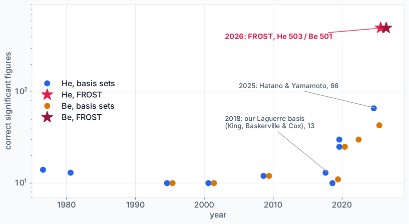
TLDR: In this post learn how to calculate the Hartree–Fock energy of helium to 503 significant figures and of beryllium to 501, both as rigorous upper bounds, on one core of a laptop and without a basis set. The previous records were 66 and 43. The trick is to stop expanding the orbital in a basis, solve the Hartree–Fock equations directly with Taylor series of order up to 873, and then check the answer with a separate program that uses nothing but integer arithmetic.
This post is part of a series on Hartree-Fock theory:
- Restricted Hartree-Fock in 100 Lines: The original post; start here if new to HF
- Unrestricted Hartree-Fock in 100 Lines: Open shells and spin contamination
- The Integrals at the Heart of Hartree-Fock Theory: Every integral the basis-set approach needs, derived from scratch
- Hartree–Fock to 500 Significant Figures with FROST: You are here, and we throw the basis set away
The result (in hartrees)
All 503 and 501 figures are written out in full in Part III and Part IV.
Introduction or an intervention? No, I have not lost my mind, I promise
A couple of months ago I wrote about FLAKE, a method that computed the exact non-relativistic ground-state energy of helium to 60 significant figures and I spent a good chunk of that post arguing that nobody needs that many digits, so why here am I going to 500+ digits for Hartree Fock? Before sectioning me under the Mental Health Act hear what I have to say as this is an idea I have had for years and wanted to finally realise it.
The first reason is the same as last time, the method is the interesting part. Getting hundreds of digits forces you to understand exactly where every error comes from or to approach the problem in an entirely different way. You cannot hide anything behind a convergence plot that “looks flat”.
The second reason is new, FLAKE and FROST are not two separate obsessions, they are two halves of the reference data for another project I have been working on in the background. That project needs two-electron atoms whose energy, orbitals and density are known essentially exactly, with an error bar at every point in space, not just a number at the end.
This new idea deserves its own post so I will not say more yet, but here is a teaser. Subtract the Hartree–Fock energy from the exact energy and you get what Löwdin called the correlation energy, the part of the electron–electron interaction that a single Slater determinant cannot describe. Combining FLAKE and FROST gives, for helium,
Its accuracy is now set entirely by FLAKE; the Hartree–Fock side has more than 400 figures to spare; make of that what you will.
In keeping with the frozen theme of FLAKE, I have called the new method FROST: Fock Radial Orbital Shooting with Taylor series where every word is doing a job, which we will see as we go through the post. I had also thought of ice-cream related names due to FLAKE, but I feel cold, winter wastelands devoid of life are very in keeping with quantum chemistry.
Try the code yourself
All of the code lives in FROSTCode/. You need Python 3 and gmpy2 (pip install gmpy2), plus matplotlib for the figures. Times are for one core of an Apple M4 Pro.
| file | what it does |
|---|---|
oracle.py | the helium-like solver (one orbital), 190 lines |
oracle_ns.py | the same method for several \(s\) orbitals (beryllium) |
certify.py | the independent exact-integer certificate, shares no code with the solvers |
properties.py | exact cusp, \(\rho(0)\), \(\langle r^k\rangle\) and kinetic energy of the certified orbitals |
test_hf_taylor.py | end-to-end check of everything above (~50 s) |
he_like_series.txt | certified energies for \(Z = 1\) to 10, to 100 significant figures |
make_figures.py | every figure in this post (reads the run summaries in data/) |
1
2
3
4
5
6
python oracle.py --digits 120 --out he.json      # 11 s, helium
python certify.py he.json                         #  3 s, the bound
python properties.py he.json                      #  1 s, cusp, <r^k>
python oracle.py --Z 3 --digits 100 --out li.json # Li+, or any Z
python oracle_ns.py --Z 4 --digits 100 --out be.json  # ~3 min
python certify.py be.json
The 500-digit results are the same commands with --digits 500. That takes about 8 minutes for helium and 4 hours for beryllium.
Birds-eye view
- Part I sets up Hartree–Fock, the standard way of computing it, and the history of the record
- Part II is the method in full detail. If you only want to know how to implement FROST, read this part
- Part III is the helium-like results, including H\(^-\) and why this was so much easier than FLAKE
- Part IV extends the method to beryllium, where things get more interesting
- Part V asks whether the orbital is as good as the energy (it is)
- Part VI is the list of things that broke on the way, and Part VII the lessons
Part I: Hartree–Fock, and how everyone computes it
1. What Hartree–Fock is
I have covered the mechanics in the RHF in 100 lines post, so here is the short version. Hartree–Fock (HF) approximates the many-electron wavefunction by a single Slater determinant of one-electron orbitals. Each electron then moves in the average field of all the others, and the orbitals must be consistent with the field they produce, hence “self-consistent field”. It is a variational method meaning the HF energy is the lowest energy any single determinant can have, so it is always above the exact energy.
For the ground state of helium, both electrons sit in the same spatial orbital \(\phi(\mathbf r)\), one spin up and one spin down. That is the closed-shell \(1s^2\) configuration. In atomic units the energy of a normalised orbital is
\[E_{\rm HF} = 2\langle\phi\vert -\tfrac12\nabla^2 - \tfrac{Z}{r}\vert\phi\rangle + (\phi\phi\vert\phi\phi),\]two one-electron energies plus the Coulomb repulsion between the two electron clouds. The HF orbital minimises this, and the HF limit is that minimum, the exact solution of the HF equations with no basis-set error at all; that is the number this post is about.
Like the FLAKE number, it is not physical past the first few digits: HF is a model, and nature does not do mean fields, but it is a perfectly well-defined mathematical number. It is the reference against which correlation is measured, and the standard test of every numerical HF method and basis set ever written.
2. The standard recipe: choose a basis
Almost every HF calculation since 1951 follows Roothaan’s recipe:
- Pick a basis \(\lbrace\chi_\mu\rbrace\) and expand \(\phi = \sum_\mu c_\mu\chi_\mu\)
- Compute the overlap, one-electron and two-electron integrals over the basis. There are \(O(N^4)\) of the last kind
- Solve the Roothaan–Hall equations \(\mathbf F\mathbf c = \varepsilon\mathbf S\mathbf c\), rebuild \(\mathbf F\) from the new \(\mathbf c\), and repeat until self-consistent
- Make the basis bigger and repeat, to see how close you are to the limit
The whole art lies in step 1. Slater-type orbitals \(r^n e^{-\zeta r}\) (Clementi and Roetti’s famous tables), Gaussians (pretty much everyone else), B-splines, finite elements and Laguerre functions have all been tried. In 2018 we did HF for two-electron atoms with a Laguerre basis in perimetric coordinates. The two-electron integrals needed the 7-nested summation I wrote about last year, and the energy was good to 13 significant figures.
For atoms there is also numerical HF, which Charlotte Froese Fischer turned into the standard tool, where yuo solve the radial HF equations on a grid with finite differences. That avoids the basis but is limited by the order of the difference scheme and, in practice, by double precision.
3. A century of chasing Hartree–Fock digits
Correct significant figures of the HF energies of helium and beryllium (log scale). For four decades nothing moved past 14 figures.
| Year | Who | Method | He (s.f.) |
|---|---|---|---|
| 1977 | Gázquez & Silverstone | piecewise polynomials | 14 |
| 1995 | Koga et al. | Slater-type functions | 10 |
| 2009 | Saito | B-splines | 12 |
| 2018 | King, Baskerville & Cox | Laguerre basis, perimetric coordinates | 13 |
| 2019 | Lehtola | finite elements | 10 |
| 2020 | Cinal | pseudospectral, quadruple precision | 25 |
| 2020 | Hatano & Yamamoto | Laguerre-type \(\Lambda\) functions, quadruple precision | 30 |
| 2025 | Hatano & Yamamoto | \(\Lambda\) functions, multiple precision | 66 |
| 2026 | this work | FROST: no basis, exact-integer certificate | 503 |
These values are a selection from Table 4 of Hatano and Yamamoto’s 2025 paper (the figure shows all of them), each truncated to its correct figures. The striking thing is the plateau. From the 1970s to 2019 every method, whatever its basis, landed at 10 to 14 figures. That ceiling is set largely by double-precision arithmetic, which holds about 16 digits, and the basis-set error was never the bottleneck. Quadruple precision lifted it to 25 and 30. Hatano and Yamamoto then moved their \(\Lambda\)-function calculation to multiple precision: 150 functions with a single optimised exponent, integrals accurate to 80 digits, and 66 correct figures. That was the record until now. Beryllium tells the same story, ending at 43.
4. Why basis sets run out of steam
Two obstacles stand between a basis-set method and hundreds of digits.
The integrals. The number of two-electron integrals grows as \(N^4\), and every one must be computed to more than the target precision. The SCF iterations then need linear algebra on ill-conditioned matrices at that precision too.
The orbital itself. This is the more fundamental one, and it is the most surprising thing I learned on this project. The HF orbital of helium has singularities in the complex plane, close to the nucleus. We will find them in §9 and see in §14 that they force any single-exponent basis to converge sub-geometrically. Extrapolating the record calculation to 500 digits would need about 2,800 basis functions and something like \(10^{13}\) two-electron integrals at 500-digit precision. That is a hard no on a laptop.
So instead of trying to build a better basis, FROST does not use one.
Part II: FROST, the method in full
Hartree Fock was not part of the curriculum during my MPhys degree, and when I learned about the Roothan-Hall equations during my PhD I always had this nagging question, more issue; you need a basis set, but is this a necessity, or just one way of representing the problem?
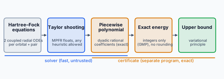 Two programs. The solver (blue) can use any arithmetic and any heuristic it likes. The certificate (amber) only sees an explicit function and evaluates its energy exactly.
The one-sentence version:
For atoms whose occupied orbitals are all \(s\) orbitals, the HF equations are ordinary differential equations in \(r\). Solve them directly with Taylor series to any order, then treat the result as an explicit trial function and evaluate its energy in exact integer arithmetic.
We now go through it one step at a time, for helium first. Beryllium is Part IV.
5. Hartree–Fock for 1s² as two ODEs
FIrst we write the orbital as \(\phi(\mathbf r) = f(r)/\sqrt{4\pi}\), so that normalisation is \(\int_0^\infty f^2r^2\,dr = 1\). Both electrons sit in the same spatial orbital \(\phi(\mathbf r)\), one with each spin. Because a 1s orbital is spherical, it is a radial function times the constant spherical harmonic \(Y_{00} = 1/\sqrt{4\pi}\), so we write \(\phi(\mathbf r) = f(r)/\sqrt{4\pi}\). Here \(f(r)\) is the ordinary radial function \(R_{1s}(r)\), not the \(P(r) = rR(r)\) used in many numerical HF codes. It is normalised as \(\int_0^\infty f^2r^2,dr = 1\). As a mental picture, \(f\) looks much like the screened hydrogenic \(2\zeta^{3/2}e^{-\zeta r}\) with \(\zeta = 27/16\).
For an unnormalised radial function the closed-shell HF energy is
\[E[f] = \frac{2(T+V)}{N} + \frac{J}{N^2},\] \[N = \int_0^\infty f^2r^2\,dr,\quad T = \frac12\int_0^\infty f'^2r^2\,dr,\quad V = -Z\int_0^\infty f^2r\,dr,\quad J = 2\int_0^\infty f^2\,r\,Q(r)\,dr,\]where \(Q(r) = \int_0^r f^2s^2\,ds\) is the charge of one electron inside radius \(r\). \(J\) is the Coulomb repulsion \((\phi\phi\vert\phi\phi)\): for spherical charge clouds, Gauss’s law turns the six-dimensional two-electron integral into a one-dimensional one. There are no two-electron integrals in the usual sense anywhere in this post which is rather pleasing.
For \(1s^2\) the exchange term cancels exactly half of the Coulomb term, so the Fock operator is just \(-\tfrac12\nabla^2 - Z/r + V_{\rm H}(r)\), where \(V_{\rm H}\) is the electrostatic (Hartree) potential of one electron. Two things to write down:
- The HF equation. \(-\tfrac12\big(f''+\tfrac2rf'\big) - \tfrac Zrf + V_{\rm H}f = \varepsilon f\)
- Poisson’s equation for \(V_{\rm H}\), with the charge density \(f^2/4\pi\) of one electron
Now the key substitution: \(Y(r) = r\,V_{\rm H}(r)\). Multiply the HF equation by \(-2r\), and write Poisson’s equation with the radial Laplacian \(\nabla^2V_{\rm H} = \frac1r(rV_{\rm H})'' = -f^2\). The result is the pair
\[\boxed{\;r f'' + 2f' = 2\,(Y - Z - \varepsilon r)\,f, \qquad Y'' = -r f^2\;}\]The boundary conditions are:
- \(f\) is regular at the origin and decays at infinity
- \(Y(0) = 0\) at the nucleus
- \(Y\to 1\) and \(Y'\to0\) at infinity, which is Gauss’s law: far away, one electron’s potential is \(1/r\)
The total energy follows from the orbital energy as \(E = 2\varepsilon - J\).
That is the entire problem; two coupled, nonlinear ODEs with an eigenvalue, no matrices, no basis and no SCF loop. The self-consistency is built in, because \(Y\) is integrated alongside \(f\) from the same equations.
6. A cheeky degeneracy
To integrate outward from \(r = 0\) we need everything at the origin. Since \(f\) is regular there, the HF equation fixes \(f'(0)\) from \(f(0)\) (more in §8), and \(Y(0)=0\). That leaves three unknown numbers: \(a = f(0)\), \(b = Y'(0) = V_{\rm H}(0)\) and \(\varepsilon\).
But if we look at Poisson’s equation: \(Y'' = -rf^2\) does not involve \(b\) at all. So we can split off the linear part exactly, \(Y = b\,r + \tilde Y\) with \(\tilde Y(0) = \tilde Y'(0) = 0\). Then
\[Y - \varepsilon r = \tilde Y - (\varepsilon - b)\,r = \tilde Y - \mu r, \qquad \mu = \varepsilon - b,\]and the orbital depends on \(b\) and \(\varepsilon\) only through their difference \(\mu\). A constant shift of the potential is the same thing as a shift of the energy. If you shoot in \((a, b, \varepsilon)\) the Jacobian is exactly singular, and any Newton-type solver will wander. Shooting in \((a, \mu)\) instead, the two conditions at the far end are
\[f(R) = 0, \qquad N(R) \equiv \tilde Y(R) - R\,\tilde Y'(R) = 1 .\]The second is the normalisation in disguise, because \(\frac{d}{dr}(\tilde Y - r\tilde Y') = -r\tilde Y'' = r^2f^2\). So we get \(\int_0^R f^2r^2\,dr\) for free from the potential. Once these are met, \(Y'(R) = 0\) fixes \(b = -\tilde Y'(R)\) and \(\varepsilon = \mu + b\).
7. The wall
We cannot integrate to infinity (although in some of my very old helium expectation value codes I defined infinity to be 100 so technically I could integrate to infinity!), so we put a hard wall at radius \(R\). That means imposing \(f(R) = 0\) and setting \(f = 0\) beyond it. This is the only approximation in the whole method, and it is a variational one. Orbitals confined to \([0, R]\) are a subset of all admissible orbitals, so the confined minimum satisfies \(E_R \ge E_{\rm HF}\).
How big is the error? Far from the nucleus the orbital sees the residual Coulomb field \(-(Z-1)/r\) and decays as \(f\sim r^{\sigma-1}e^{-\kappa r}\), with \(\kappa = \sqrt{-2\varepsilon}\) and \(\sigma = (Z-1)/\kappa\). The energy error is set by the squared amplitude at the wall,
\[E_R - E_{\rm HF} \simeq C\,R^{2\sigma}e^{-2\kappa R}.\]For helium \(\kappa = 1.354958\), so every bohr of wall buys \(2\kappa/\ln 10 = 1.18\) significant figures. For \(D\) digits we place the wall at \(R = (D+8)\ln 10/(2\kappa)\): 109 bohr for 120 digits, 432 bohr for 500. In Part III we check this law against the computed energies, and it predicts the 500-digit error to 1% from walls no bigger than 100 bohr.
8. Taylor series of any order
This is the engine powering the entire method, about any point \(r_0\), write \(f = \sum_k f_k(r-r_0)^k\) and similarly for \(\tilde Y\). Products of series become Cauchy convolutions, \((uv)_k = \sum_{j\le k}u_jv_{k-j}\). Equating powers of \((r-r_0)\) in the two ODEs gives explicit recurrences (recurrences are still magic to me and I love trying to use them to solve problems):
\[\begin{aligned} \tilde Y_{k+2} &= -\frac{r_0(f^2)_k + (f^2)_{k-1}}{(k+1)(k+2)},\\ f_{k+2} &= \frac{g_k - (k+1)(k+2)f_{k+1}}{r_0(k+1)(k+2)}, \qquad g_k = 2\big[(\tilde Yf)_k - Zf_k - \mu(r_0f_k + f_{k-1})\big]. \end{aligned}\]Given the value and slope of \(f\) and \(\tilde Y\) at \(r_0\), every higher coefficient follows, and order \(p\) costs \(O(p^2)\) multiplications. In code this is a dozen lines (simplified from oracle.py, which also carries the energy integrals along as two more series):
1
2
3
4
5
6
7
8
9
10
11
12
13
14
15
16
17
18
19
20
21
def dot(a, b):
    """One Cauchy-product coefficient, sum_i a[i] b[n-1-i]."""
    return sum(x * y for x, y in zip(a, reversed(b)))

def series(r0, f0, df0, Y0, dY0, mu, Z, p):
    """Order-p Taylor coefficients of f and Y~ about r0.
    At r0 = 0 (Y0 = dY0 = 0) it is the Frobenius series; df0 unused."""
    f = [f0] if r0 == 0 else [f0, df0]
    Y, ff = [Y0, dY0], []
    for k in range(p):
        prev = lambda c: c[k - 1] if k else 0      # c_(k-1), 0 at k = 0
        m = (k + 1) * (k + 2)
        ff.append(dot(f[:k + 1], f[:k + 1]))       # (f^2)_k
        Y.append(-(r0 * ff[k] + prev(ff)) / m)
        g = 2 * (dot(Y[:k + 1], f[:k + 1]) - Z * f[k]
                 - mu * (r0 * f[k] + prev(f)))
        if r0 == 0:                                # regular singular point
            f.append(g / m)
        else:
            f.append((g - m * f[k + 1]) / (r0 * m))
    return f, Y
All arithmetic is in MPFR floating point via gmpy2, at whatever precision we ask for: 1,827 bits for the 500-digit runs. I normally pile in on how crap MPFR is, but it works fine here and is the path of least resistance to a solution so I tolerate it.
The nucleus comes for free. At \(r_0 = 0\) the equation has a regular singular point. Expanding \(rf''+2f'\) there, the power \(r^k\) picks up \((k+1)(k+2)f_{k+1}\), so only \(a = f(0)\) is free. The singular solution \(\sim 1/r\) is excluded automatically. The very first step of this Frobenius recurrence is
\[f_1 = \frac{g_0}{2} = \frac{2(0 - Z)f_0}{2} = -Z f_0,\]which is Kato’s cusp condition, built into the recurrence! Basis-set methods have to approximate the cusp, and smooth bases like Gaussians never get it right. Here it is exact. For \(Z = 2\) and \(Z = 4\), multiplying by \(Z\) does not even round, so the certified orbital’s \(f'(0)/f(0)\) is exactly the rational number \(-Z\) (Part V).
The higher Frobenius coefficients also come from the HF equation itself, so the orbital has the analytic form of the true HF solution at the nucleus, not just the right slope. If you have ever fought a cusp with Gaussians, this is quite satisfying.
9. Letting the orbital choose its own steps
A Taylor series about \(r_0\) converges inside a disc whose radius is the distance to the nearest singularity of the solution. Inside it, truncating at order \(p\) with step \(h = c\rho\) costs a relative error of about \(c^p\). So we:
- estimate the radius of convergence \(\hat\rho\) from the coefficients themselves, using the root test on the last nine, \(\hat\rho = \min_{p-8\le k\le p}\vert f_0/f_k\vert^{1/k}\);
- take the step \(h = c\,\hat\rho\), with \(c = 0.15\) by default;
- choose the order \(p = \lceil (d+5)/\log_{10}(1/c)\rceil\) for \(d\) target digits, so that \(c^p\) is below the working precision.
1
2
3
4
5
6
7
def step_size(f, c):
    """c times the radius of convergence (root test on the last 9
    coefficients), rounded DOWN to a multiple of 2^-16."""
    p = len(f) - 1
    rho = min((abs(f[0]) / abs(f[k])) ** (1 / k)
              for k in range(p - 8, p + 1) if f[k])
    return floor(c * rho * 2**16) / 2**16
The rounding to a \(2^{-16}\) grid looks like a detail, but it matters later: every knot of the mesh is an exact dyadic rational (I grew up in Chatham and Maidstone in the UK so am unapologetically. What I meant to say is every knot can be written as a fraction with an integer numerator and a power of two as the denominator… init bruv), which the certificate needs (§13).
What does the radius look like along the orbital?
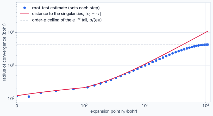 Blue: the root-test estimate at every step of the 120-digit run. Red: the distance from \(r_0\) to a pair of complex singularities at \(r_* = -1.099\pm0.577i\). Dashed: beyond ~20 bohr a finite order sees the \(e^{-\kappa r}\) tail’s coefficients \(\kappa^k/k!\) first, which caps the estimate.
The radius grows linearly with distance from the nucleus. That is what you get if it is the distance to a fixed singular point. The hydrogen orbital \(e^{-Zr}\) has no singularities anywhere (it is entire), but the HF equations are nonlinear and their solutions can have movable singularities. Fitting the sign pattern of the 626th-order Frobenius series at \(r = 0\) (it rotates with \(k\), the signature of a complex-conjugate pair) puts them at
\[r_* = -1.099 \pm 0.577\,i, \qquad \vert r_*\vert = 1.241 \text{ bohr}.\]Fits about \(r_0 = 0.6, 1.5, 3.5, 8\) and \(17\) bohr all find the same pair. Because the radius grows linearly, the steps grow geometrically: 41 steps reach 109 bohr and 51 steps reach 432 bohr. The orbital tells us how far we can go, and we never need a fine mesh in the tail.
10. Shooting, and why the obvious solver fails
For given \((a, \mu)\) we can now integrate from 0 to \(R\). We need the pair for which \(f(R) = 0\) and \(N(R) = 1\). This is a shooting problem, and the far end is where the danger lives.
Away from the nucleus the HF equation has two solutions, one decaying as \(e^{-\kappa r}\) and one growing as \(e^{+\kappa r}\). If \(\mu\) is wrong by a relative \(\delta\), the integrated orbital carries the growing solution with an amplitude proportional to \(\delta\). It overtakes the true orbital at around \(r \approx \ln(1/\delta)/2\kappa\):
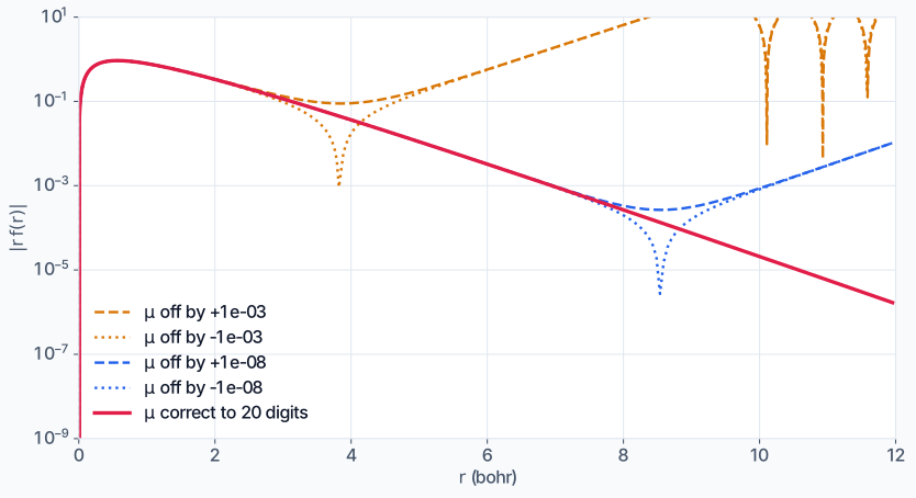 Get \(\mu\) wrong by \(10^{-8}\) and the orbital is ruined beyond 8 bohr. The sign of the error decides which way it blows up (the dips are where \(f\) crosses zero). For 500 digits at 432 bohr, \(\mu\) has to be right to about 500 digits.
That sensitivity is exactly what makes \(\mu\) easy to find: \(f(R)\) is almost perfectly linear in \(\mu\), because \(\mu\) just sets the amplitude of the growing mode, a secant iteration converges in two or three integrations.
The natural thing to do with two unknowns and two conditions is a joint \(2\times2\) Newton iteration. It fails at large \(R\) because away from the solution the normalisation \(N(R)\) contains the growing mode squared, a term proportional to \(e^{2\kappa R}\). Its Jacobian row therefore lines up with that of \(f(R)\). At \(R = 277\) in a 500-digit run the two rows were parallel to 31 digits, and the basin of convergence of the joint iteration shrinks as \(e^{-\kappa R}\).
The fix is to nest two scalar problems:
1
2
3
4
5
6
7
8
9
10
11
12
# simplified from oracle.py; shoot() integrates 0 -> R
# and returns f, Y~ and Y~' at the wall
def stage(a, mu, R):
    def norm(a):
        """Outer residual N(R) - 1, with mu re-solved for this a."""
        nonlocal mu
        # inner solve, f(R) = 0: two or three shots
        mu = secant(lambda m: shoot(a, m, R).f, mu)
        s = shoot(a, mu, R)
        return s.Y - R * s.dY - 1
    a = secant(norm, a)
    return a, mu
Every evaluation of the outer residual first solves for \(\mu\), so no growing mode is ever left in \(N\). The outer function \(N(a)\) is then smooth, and a secant on \(a\) converges quickly. Within a stage the mesh is frozen (computed once, then reused), so both residuals are smooth functions of the unknowns rather than jumping whenever a step size changes.
Lesson. When one residual contains a growing mode, do not solve it jointly with anything. Solve it first, inside, so the other residuals never see it.
11. Continuation
Shooting needs a decent starting guess, and a wall at 432 bohr is far too sensitive to start cold. So we crawl out to it instead:
- Start from a screened hydrogenic orbital, \(\zeta = Z - 5/16\), with a small wall \(R_0 = 7/\zeta\)
- Solve, multiply \(R\) by 1.2 (on a \(1/64\) grid), and use the solution as the next starting point
- At each stage, target only the \(d_k = \min(D, 2\kappa R_k/\ln10) + 10\) digits that this wall can deliver, with working precision \(d_k + 40\) digits, and update \(\kappa\) from the current \(\varepsilon\)
After the first few stages, which take up to 60 integrations from the hydrogenic start, every stage takes 15 to 23 integrations, independent of \(R\). Precision and order grow as the wall moves out, so the early stages are almost free.
12. Isn’t a piecewise polynomial just a basis, got’em, I hear you cry?
We write the orbital to disk as a polynomial on each step, and a piecewise polynomial certainly could be a basis, finite elements and B-splines are both piecewise polynomials.
The difference is in what is unknown. In a basis-set calculation, including finite elements, the coefficients of fixed functions are the unknowns. They come from integrals and a matrix eigenproblem, and the accuracy is limited by how well those functions can represent the orbital, which is what all the effort goes into.
In FROST no coefficient is an unknown. Given the two numbers \(a\) and \(\mu\), the recurrence of §8 fixes every coefficient. The polynomial on each step is the local Taylor expansion of the true solution, truncated where its remainder falls below the working precision, and the mesh is chosen by the solution’s own radius of convergence. Nothing is optimised over the polynomial, and its representation error is never what limits the result. Like any high-order ODE integrator, the method produces a piecewise polynomial. It is a by-product, not a design choice, but it is an extremely useful one because of what we can do with it next.
13. Certification with integers only
The solver’s energy is accurate but not rigorous because it is affected by rounding, series truncation and the secant tolerance. I learned with FLAKE that the solver’s number is not the result, so FROST has a separate program, certify.py, about 180 lines, that shares no code with the solver. Its job is to turn the solver’s output into a variational upper bound with no arithmetic error at all (the dream).
The idea relies on one fact about binary floating point: every MPFR number is a dyadic rational (init bruv), \(m\cdot2^e\) with integer \(m\) and \(e\). The solver writes each coefficient as the exact pair \((m, e)\), and the knots lie on the \(2^{-16}\) grid. So the solver’s orbital is, exactly, a piecewise polynomial with rational coefficients. The certificate then:
- Checks the mesh exactly. The elements must tile \([0, R]\): \(r_0 = 0\), \(h_j>0\) and \(r_j + h_j = r_{j+1}\), all compared as exact rationals. A reversed interval would fake a lower “bound”, so this is not optional
- Maps each element to \([0, 1]\) with \(r = r_j + h_js\), and multiplies everything by one common power of two so that every polynomial has integer coefficients. The energy functional is scale invariant, so nothing changes
- Imposes continuity and the wall exactly. It sets each element’s constant term equal to the previous element’s value at \(s = 1\), and adjusts the last element’s linear coefficient so that \(f(R) = 0\). These adjustments are the size of the solver’s residuals, about \(10^{-d}\). With \(f = 0\) beyond \(R\) the trial function is continuous with finite kinetic energy, so it is admissible
- Integrates exactly. On each element every integrand in \(N, T, V, J\) is an integer polynomial in \(s\), and its integral over \([0,1]\) is a fraction with denominator \(\mathrm{lcm}(1,\dots,n)\). The inner integral \(Q(r)\) is carried across elements as an exact antiderivative
- Forms \(E[f]\) as one rational number and prints it rounded towards \(+\infty\)
1
2
3
4
def pint(a):
    """int_0^1 a(s) ds for an integer polynomial a, exactly."""
    L = lcm_to(len(a))                    # lcm(1, ..., n)
    return mpq(sum(c * (L // (k + 1)) for k, c in enumerate(a)), L)
The variational principle then gives
\[E_{\rm HF} \;\le\; E_R \;\le\; E[f]\]with no rounding anywhere. Note what this means: any piecewise polynomial would produce a valid bound. The solver can use any arithmetic, any heuristic and any step size it likes, and if it has a bug the bound gets worse, not wrong. Its only job is to make the bound tight.
The one optimisation that mattered. Almost all of the certificate’s time goes into multiplying integer polynomials of degree around \(2p\) whose coefficients are thousands of bits long. The schoolbook double loop in Python is slow. The trick is Kronecker substitution: pack each polynomial into a single huge integer, with each coefficient in its own fixed-width slot, multiply the two integers once with GMP’s fast multiplication, and unpack. A toy example in base 1000:
\[(3x+2)(4x+1)\;\to\; 3002\times4001 = 12\,011\,002 \;\to\; 12x^2 + 11x + 2 .\]The slots just need to be wide enough that no coefficient of the product overflows into its neighbour. Negative coefficients are handled by splitting each polynomial into positive and negative parts. It returns bit-identical rationals 4 to 5 times faster. The 120-digit helium certificate takes 3 seconds; the 500-digit one, before this trick, took 34 minutes.
As far as I can tell nobody has done this for HF before, but if they have message me. The closest earlier work I could find is Janes and Rendell’s interval-arithmetic bounding of rounding errors in basis-set HF, which is a different thing.
14. What the singularities say about basis sets
Now we can come back to the question from §4, why do basis sets struggle so much? The record calculations use Laguerre-type functions \(L^{(2)}_n(2\zeta r)e^{-\zeta r}\) with one exponent \(\zeta\), and our 2018 basis was of the same kind. Expanding \(f\) in them amounts to expanding \(g(x) = f(x/2\zeta)\,e^{x/2}\) in Laguerre polynomials. Two features of the orbital limit how fast the coefficients fall:
- The tail. The true tail \(e^{-\kappa r}\) does not match the basis exponent. From the Laguerre generating function, its coefficients fall as \(t^n\) with \(\vert t\vert = (\zeta-\kappa)/(\zeta+\kappa)\). You want \(\zeta\) close to \(\kappa\)
- The singularities. A Laguerre series converges inside the largest parabola \(\mathrm{Re}\sqrt{-x} < \tau\) that avoids every singular point, with coefficients falling as \(e^{-2\tau\sqrt n}\). The singular points \(r_*\) map to \(x_* = 2\zeta r_*\), giving \(\tau = 1.0815\sqrt{2\zeta}\). You want \(\zeta\) large
The two pull in opposite directions. Balancing them gives an optimal exponent \(\zeta_{\rm opt}\propto N^{1/3}\) and an error \(\exp(-cN^{2/3})\), which is slower than any geometric rate.
This crude estimate ignores all prefactors, so I did not expect much from it. For \(N = 150\) it predicts \(\zeta_{\rm opt} = 4.98\), and Hatano and Yamamoto’s numerically optimised exponent is 5.1448, within 3%. At their exponent the two mechanisms limit the energy to about 70 and 74 digits, so their optimiser had found the balance point, and the 66 digits they observed fit. On the same estimate, 503 digits would need \(N\approx2{,}800\) functions with \(\zeta\approx13\).
Taylor steps do not care about any of this as each one converges geometrically inside its own disc, and the disc sizes are set by the very singularities that cripple the global expansion.
Part III: Results for two electrons
Helium
| run | digits | wall (bohr) | order | steps | solver | certificate | correct s.f. |
|---|---|---|---|---|---|---|---|
| A | 120 | 108.77 | 164 | 41 | 11 s | 3 s | 124 |
| B | 500 | 431.66 | 626 | 51 | 7.4 min | 34 min | 503 |
| C | 500 | 445.00 | 856 | 30 | 8.2 min | reference |
Runs B and C are independent: different walls, orders, step fractions (\(c = 0.15\) and \(0.25\)), meshes and working precisions (1,827 and 1,793 bits). Run A’s certificate time is for the current code; run B’s was measured before the Kronecker speed-up of §13. The certificate of run B gives a rigorous upper bound. Here are all 503 correct figures:
How do we know 503 of them are correct? The bound is rigorous, so the only question is how far above \(E_{\rm HF}\) it lies.
- Run B lies \(1.70\times10^{-503}\) above run C.
- The wall law of §7, with \(C\) fitted only to walls between 20 and 100 bohr, predicts \(1.69\times10^{-503}\) for run B’s wall. So the whole difference is run B’s wall error, and the law extrapolated over 400 digits to get there.
- Run C’s own wall error is about \(10^{-519}\), and its truncation and rounding are set below that.
So the bound lies \(1.70\times10^{-503}\) above the HF limit, a relative error of \(10^{-503.2}\).
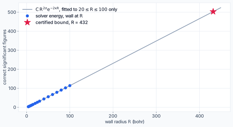 The wall law, fitted on the blue points up to \(R = 100\), predicts the 500-digit run to 1%.
Two more internal checks. The virial theorem says the energy is minus the total kinetic energy, \(E = -T_{\rm tot}\), and run B satisfies it to \(\vert E + T_{\rm tot}\vert = 2.0\times10^{-500}\). That looks like a failure until you remember that a wall exerts a pressure, which adds a term to the virial theorem. The ratio of the virial gap to the wall error is 1168, and the pressure term predicts \(2\kappa R = 1170\). And all 66 figures of Hatano and Yamamoto agree with ours.
The isoelectronic series
It wouldn’t be a two-electron blog post without an isoelectronic series table. Only \(Z\) changes along the series, so the same code gives every two-electron atom. Each line below is a certified 100-digit run (10 to 16 s plus a certificate), compared with an independent run with a larger wall. Every bound lies above its reference and agrees with it to 103 to 108 figures. The full 100-digit values are in he_like_series.txt.
| \(Z\) | ion | \(E_{\rm HF}\) (hartree) | wall (bohr) | agreement (s.f.) |
|---|---|---|---|---|
| 1 | H\(^-\) | −0.4879297343708517486928383… | 409.0 | 107.8 |
| 2 | He | −2.861679995612238878775543… | 91.8 | 104.2 |
| 3 | Li\(^+\) | −7.236415201452256247682907… | 52.6 | 103.7 |
| 4 | Be\(^{2+}\) | −13.61129943061910903495583… | 36.9 | 103.5 |
| 5 | B\(^{3+}\) | −21.98623446682434301967704… | 28.5 | 103.3 |
| 6 | C\(^{4+}\) | −32.36119287571801233131520… | 23.2 | 103.3 |
| 7 | N\(^{5+}\) | −44.73616396494247312978203… | 19.5 | 103.3 |
| 8 | O\(^{6+}\) | −59.11114270191365385859847… | 16.9 | 103.2 |
| 9 | F\(^{7+}\) | −75.48612640626050983759562… | 14.9 | 103.2 |
| 10 | Ne\(^{8+}\) | −93.86111351923133815497816… | 13.3 | 103.2 |
As \(Z\) grows the orbital is more tightly bound, \(\kappa\) grows, and the wall needed for 100 digits shrinks from 409 bohr for H\(^-\) to 13 bohr for Ne\(^{8+}\).
The hydrogen anion, which Hartree–Fock says should not exist
You will often read (or hear from me) that H\(^-\) is “unbound in Hartree–Fock”. So how is it in the table?
What the phrase means is that \(E_{\rm HF}({\rm H}^-) = -0.48793\) lies 0.0121 hartree above the energy of a hydrogen atom plus a free electron, \(-\tfrac12\). HF predicts a negative electron affinity, which is wrong. Real H\(^-\) is bound, and the binding is entirely a correlation effect.
But the closed-shell HF problem itself still has a perfectly good normalisable solution. At large \(r\) the Hartree potential \(Y/r\to1/r\) cancels the nuclear attraction exactly, so the orbital sees a short-range potential well that is deep enough to bind it. The orbital energy is \(\varepsilon = -0.04622\ldots\), and \(f\sim e^{-0.304 r}/r\).
The calculation shows this directly: \(\varepsilon\) converges to 15 digits by \(R\approx76\) bohr and then does not move as the wall goes out to 409 bohr. An orbital held in place only by the wall would have \(\varepsilon\to0\) as \(R\) grows. What keeps the ion together is the closed-shell constraint. Without it, a determinant with one electron in H(\(1s\)) and the other spread out to infinity approaches \(-\tfrac12\), and unrestricted HF collapses to that. H\(^-\) is also the expensive member of the family: \(\kappa\) is small, so each significant figure costs 3.8 bohr of wall against 0.85 for helium.
Cost
I find the computational cost of this method incredible. Everything runs in Python with gmpy2 on one CPU core of an Apple M4 Pro.
- Solver. Each integration costs \(O(p^2)\) multiplications per step at \(d\)-digit precision, with \(p\propto d\) and \(O(\log R)\) steps. There are \(O(\log R)\) continuation stages of about 20 integrations each. In practice: 11 s at 120 digits and 7.4 minutes at 500, scaling as about \(D^{2.6}\)
- Certificate. 3 s at 120 digits; the 500-digit one took 34 minutes before the Kronecker trick
- Memory. Negligible. The 500-digit orbital file, holding every Taylor coefficient, is 18 MB
Part IV: Beryllium, more than two electrons
Helium is the obvious target, but a method that only works for one orbital is a curiosity. Beryllium, \(1s^22s^2\), has four electrons in two doubly occupied \(s\) orbitals. Every idea above carries over, but a few new problems appear, and they took most of the effort.
The equations
For \(n\) doubly occupied \(s\) orbitals \(f_i\), every pair of orbitals gets a potential
\[Y_{ij}(r) = r\int_0^\infty\frac{f_i(s)f_j(s)\,s^2}{\max(r,s)}\,ds, \qquad Y_{ij}'' = -r\,f_if_j .\]\(Y_{ii}\) is the Coulomb potential of orbital \(i\) and \(Y_{ij}\) (\(i\ne j\)) the exchange potential between \(i\) and \(j\). Here is the nice part: for \(s\) orbitals only the monopole term survives, so exchange is a multiplication, not an integral operator. The canonical HF equations become
\[rf_i''+2f_i' = 2\Big[\Big(\sum_j2Y_{jj}-Y_{ii}-Z-\varepsilon_ir\Big)f_i-\sum_{j\ne i}Y_{ij}f_j\Big],\]a system of ODEs just like before. The degeneracy trick of §6 also carries over: write \(Y_{ij} = b_{ij}r+\tilde Y_{ij}\), and the orbitals depend on the \(\varepsilon_i\) and \(b_{ij}\) only through combinations \(\mu_i\) and \(\nu_{ij}\). The Taylor recurrences carry over term by term, and the Frobenius series again gives \(f_i'(0) = -Zf_i(0)\) for both orbitals. Beryllium has two orbitals, three pair potentials and five shooting parameters, \((a_1, a_2, \mu_1, \mu_2, \nu_{12})\).
One wall per orbital
The \(1s\) orbital decays as \(e^{-3.077r}\) and the \(2s\) as \(e^{-0.786r}\). Put a single wall where the \(2s\) needs it and integrate the \(1s\) out there too: its growing mode \(e^{+3.077r}\) then demands about \(3.077/0.786\approx4\) times the working precision. So each orbital gets its own wall \(R_i\), chosen so that \(e^{-2\kappa_iR_i}\) is the same for both. For the 500-digit run these are 190 bohr for the \(1s\) and 744 bohr for the \(2s\). A \(1s\) that is zero beyond 190 bohr is still an admissible orbital, so the variational bound is unaffected.
Canonical, not orthogonal
With a common wall, the canonical orbitals of one Fock operator are automatically orthogonal. With unequal walls they are not, and the textbook answer is to enforce orthogonality with a Lagrange multiplier. That turned out to be badly conditioned. The overlap \(S_{12}\) responds to the multiplier only at the \(10^{-4}\) level. A Newton step big enough to correct it forces a \(1s\) tail far above its natural size, and the exchange term then feeds it straight into the \(2s\) growing mode. In one attempt the \(2s\) “normalisation” came out at 1245.
So I stopped insisting. FROST keeps the canonical equations and accepts whatever small overlap results: \(\vert S_{12}\vert = 4.9\times10^{-315}\) for the 500-digit run. The energy is stationary, so this costs only \(O(S_{12}^2)\), far below the wall error.
The certificate makes this rigorous with an old trick. For any orbitals, orthonormal or not, the closed-shell determinant energy is
\[E = 2\sum_{ij}P_{ij}h_{ij} + \sum_{ijkl}P_{ij}P_{kl}\big[2(ij\vert kl)-(ik\vert jl)\big], \qquad P = S^{-1}.\]It depends only on the span of the orbitals, so you never have to orthogonalise them. For piecewise polynomials every overlap, one-electron integral and two-electron integral is again a rational number, \(S^{-1}\) is a \(2\times2\) matrix inverted exactly, and the result is still an exact rational upper bound. For one orbital this formula reduces to the helium functional, and the generalised certificate returns the identical rational for helium.
Innermost first
Two more changes to the shooting:
- Nested solves from the inside out. Solving \(f_1(R_1)=0\) and \(f_2(R_2)=0\) jointly fails. While \(\mu_1\) is wrong, the \(1s\) carries a growing mode, exchange passes it into the \(2s\) equation, and \(f_2(R_2)\) acquires spurious roots in \(\mu_2\). So every trial \(\mu_2\) re-solves \(\mu_1\) first: the §10 lesson again, one level deeper. The outer unknowns \((a_1, a_2, \nu_{12})\) are found by Broyden’s method, with a fresh finite-difference Jacobian at each wall radius. A Jacobian carried over from the previous radius converges only linearly
- A homotopy start. A screened hydrogenic \(2s\) is too crude a starting guess. Instead, scale every electron–electron term by \(t\). At \(t = 0\) the orbitals are hydrogenic and known exactly; follow the solution to \(t = 1\) in 40 small steps at low precision
Results
| run | target digits | walls \(R_1/R_2\) (bohr) | solver | certificate | correct s.f. |
|---|---|---|---|---|---|
| A100 | 100 | 40.4 / 158.1 | 170 s | 18 s | 103 |
| A200 | 200 | 77.8 / 304.5 | 23 min | 86 s | 202 |
| A500 | 500 | 190.1 / 743.7 | 4.0 h | 13 min | 501 |
Each certified run A is checked against an independent run B with larger walls, a different step fraction and therefore a different order and mesh. The 500-digit bound lies \(7.08\times10^{-501}\) above its check run. The wall law for the \(2s\), fitted on the 100-digit run alone, predicted \(7.03\times10^{-501}\): it extrapolated across 400 digits and got within 1%. All 501 figures:
All 43 figures of the previous record agree. The orbital energies are \(\varepsilon_{1s} = -4.73266989745572620396\ldots\) and \(\varepsilon_{2s} = -0.30926955157344281760\ldots\)
Part V: Is the orbital any good?
After seeing the energies, the obvious question is whether the orbital itself is any good, or whether we just have a very accurate number.
The energy is a forgiving test. It is stationary, so an orbital error of relative size \(\delta\) changes it only at order \(\delta^2\), while every other property changes at order \(\delta\). In a basis-set calculation properties therefore carry far fewer correct figures than the energy, and fewest near the nucleus where the basis struggles with the cusp. At the 66-figure energy of the previous record, the helium cusp has 30 correct figures, \(\rho(0)\) 32 and \(\langle r^{-2}\rangle\) 35.
FROST orbitals behave differently, because their only error is the wall and that error is known in closed form. properties.py evaluates everything on the same exact trial orbitals that are certified, by exact integration of the piecewise polynomials.
The nucleus
As promised in §8, the cusp ratio \(f'(0)/f(0)\) of every certified orbital is exactly \(-Z\), both beryllium orbitals included. Not \(-1.99999\ldots\), but the rational number \(-2\). The density at the nucleus and \(\langle r^{-2}\rangle\), the properties most sensitive to this region, agree between the two independent 500-digit runs to 500 significant figures.
The pointwise error, in closed form
Once the density has decayed, \(Y = 1\) up to exponentially small terms, and the HF equation becomes the Coulomb equation for charge \(Z-1\) at energy \(\varepsilon\). Its decaying and growing solutions are Whittaker functions, \(W_{\sigma,1/2}(2\kappa r)/r\) and \(M_{\sigma,1/2}(2\kappa r)/r\). The free orbital is \(A\,W_{\sigma,1/2}(2\kappa r)/r\), and a wall at \(R\) adds exactly the multiple of the growing solution that makes \(f\) vanish there. So the relative error of the confined orbital is
\[\frac{f_R}{f}-1 \;\simeq\; -\frac{W_{\sigma,\frac12}(2\kappa R)\,M_{\sigma,\frac12}(2\kappa r)}{M_{\sigma,\frac12}(2\kappa R)\,W_{\sigma,\frac12}(2\kappa r)} \;\propto\; \Big(\frac Rr\Big)^{2\sigma}e^{-2\kappa(R-r)} .\]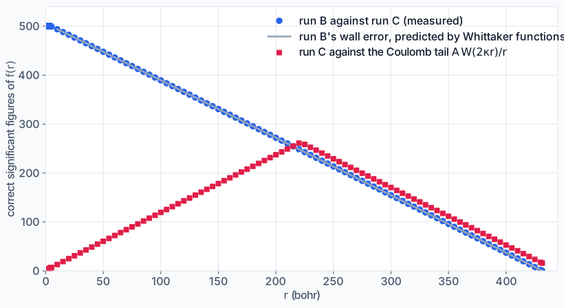 Blue: run B against run C, point by point. Grey: run B’s wall error predicted by the formula above; the two agree to one part in \(10^5\) from 10 bohr out to the wall. Red: run C against the exact Coulomb tail, which it matches to about 261 digits near \(R/2\).
So the 500-digit orbital is correct to 500 figures at the nucleus, about 250 at \(R/2\), and its error is known everywhere. The red squares also test the tail itself. Divided by \(A\,W_{\sigma,1/2}(2\kappa r)/r\), run C approaches 1 as the exponentially small part of the Hartree potential dies away, until it meets the growing wall error near \(R/2\). The decay constant, the power \(r^{\sigma-1}\) and every correction to it are those of the exact Coulomb tail. As a by-product we get the asymptotic normalisation of the helium HF orbital, \(A = 1.39080116285695292083\ldots\)
Expectation values
Because \(M_{\sigma,1/2}W_{\sigma,1/2}\) tends to a constant, the wall error changes \(f^2r^2\) by the same small amount \(u\) at every \(r\) in the Coulomb region. Then \(\delta\langle r^k\rangle\approx u\,[R^{k+1}/(k+1)-R\langle r^k\rangle]\), and each extra power of \(r\) costs about \(\log_{10}R - \log_{10}(\langle r^{k+1}\rangle/\langle r^k\rangle)\approx2\) significant figures. With \(u\) fitted at \(k = 1\), this model reproduces the run-to-run differences for every \(k\) from 1 to 12 to within 0.04%. Even \(\langle r^{12}\rangle\) is correct to 474 figures.
Per electron, against the previous record (the values are truncated to 20 figures; “s.f.” is the number of correct figures):
| helium | value | s.f. | before |
|---|---|---|---|
| cusp | \(-2\) exactly | exact | 30 |
| virial ratio \(V/T\) | \(-2\) | 500 | 68 |
| \(\rho(0)\) | 3.5959182637622489207… | 500 | 32 |
| \(\langle r^{-2}\rangle\) | 5.9955036673125245972… | 500 | 35 |
| \(\langle r^{-1}\rangle\) | 1.6872822152810094040… | 500 | 65 |
| \(\langle r\rangle\) | 0.92727340473149319741… | 497 | 63 |
| \(\langle r^2\rangle\) | 1.1848284799094829263… | 495 | 61 |
| \(\langle r^9\rangle\) | 1054.8326442597844618… | 480 | 52 |
| beryllium | value | s.f. | before |
|---|---|---|---|
| cusp | \(-4\) exactly | exact | 19 |
| virial ratio \(V/T\) | \(-2\) | 498 | 55 |
| \(\rho(0)\) | 35.387716741093786449… | 498 | 20 |
| \(\langle r^{-2}\rangle\) | 14.404506445441573899… | 498 | 23 |
| \(\langle r^{-1}\rangle\) | 2.1021994129306787940… | 498 | 41 |
| \(\langle r\rangle\) | 1.5322039722811125393… | 495 | 39 |
| \(\langle r^2\rangle\) | 4.3296928432100968739… | 492 | 38 |
| \(\langle r^9\rangle\) | 558916.88019331086049… | 478 | 30 |
Every figure the previous record prints agrees with ours.
Beryllium: the density knows more than the orbitals
Beryllium had one surprise. The two independent 500-digit runs agree on \(\rho(0)\) to 498 figures, and on the \(\langle r^k\rangle\) of the density to 478–498, which is the wall error. But the moments of the individual \(1s\) and \(2s\) orbitals agree only to 315–321 figures.
That is suspiciously close to \(\vert S_{12}\vert = 4.9\times10^{-315}\). At 200 digits the same thing happened: individual orbitals agreed to 127–133 figures with \(S_{12} = 2.6\times10^{-127}\). The explanation is that the two runs’ orbitals differ by a small rotation within the occupied space, \(1s\to1s+\theta\,2s\) and \(2s\to2s-\theta\,1s\) with \(\theta\sim S_{12}\). A determinant is unchanged by such a rotation, and so is its density, to first order. The individual orbitals are not physical; only the determinant is, and every physical property depends only on the density.
The same effect bit the kinetic energy. My first virial ratio for beryllium, at 200 digits, was good to only 127 figures, because the \(P = S^{-1}\) kinetic energy is limited by \(S_{12}\) too. Normalising each orbital on its own and summing gives 199 figures there, and 498 at 500 digits.
Part VI: Things that broke on the way
Things went wrong far less often than with FLAKE, but each failure taught me something useful, so here they are.
- The joint Newton solve. My first solver did the obvious \(2\times2\) Newton on \((a,\mu)\). It worked up to about 300 digits and then stopped converging. The cause was the parallel Jacobian rows of §10, and the fix was the nested scalar solve
- Integer walls at high \(Z\). For the isoelectronic series, walls rounded to whole bohr made the continuation jump by a factor of two at large \(Z\). The solver then happily converged to an excited state with a node and \(\varepsilon>0\). Walls on a \(1/64\) grid with \(\times1.2\) stages fixed it, along with testing convergence on the full Newton step before any damping
- Orthogonality for beryllium. Covered above; this is the one that cost the most time. The lesson was to stop enforcing a constraint the certificate does not need
- The joint inner solve for beryllium. It found spurious roots, because a wrong \(1s\) contaminates the \(2s\) through exchange. Solving innermost first fixed it
- A noise floor. The \(1s\) rounding error that remains is amplified near \(R_1\) and passed on through exchange. That limits \(\mu_2\) to about \(10^{-0.6d}\), so a scalar solve with a tight tolerance would spin forever. The energy is quadratic in orbital errors and does not care, so the solves stop when the residual stops improving
- A stale Jacobian. Reusing the outer Broyden Jacobian from the previous wall radius gave linear convergence. Recomputing it fresh at each radius is cheaper overall
- The beryllium virial ratio. Only 127 figures at first, as described in Part V
Lesson. Most of these share a root cause: a growing mode leaking into a place it should not be. If your problem has exponentially growing solutions, every design decision should be about keeping them contained.
Part VII: What transfers
Lessons
- Before choosing a basis, ask whether you need one. For \(s\) orbitals the HF problem is one-dimensional, and seventy years of basis-set tuning was solving a much harder problem than necessary
- Separate the solver from the certificate. The solver can be fast, heuristic and even buggy. The certificate is small, exact and independent. This split is what lets you trust 500 digits
- Floating-point numbers are exact rationals. Anything a floating-point solver writes down can be fed into exact arithmetic with no conversion error. That is what turns a numerical answer into a theorem
- Let the solution choose the mesh. The radius of convergence is free information sitting in the Taylor coefficients, and using it made the steps grow geometrically
- Remove exact degeneracies from the parametrisation. One line of algebra (\(\mu = \varepsilon - b\)) fixed an ill-conditioning that no solver tweak could
- Nest the solve so growing modes never reach the outer problem. This came up three times in different disguises
- Test the error model by prediction. The wall law fitted at 100 digits predicted the 500-digit errors for helium and beryllium to 1%. A model that predicts what it was not fitted to is the strongest evidence you have
- The energy is the most forgiving property. Check the orbital too; that is where basis-set errors hide
- Know your analytic structure. Two complex numbers, \(-1.099\pm0.577i\), explain both why Taylor steps work and why Laguerre bases converge slowly, and they predicted the previous record’s optimised exponent to 3%
For readers from other fields
- High-order Taylor methods for ODEs are an old idea (Moore, Corliss and Chang, Jorba and Zou’s
taylorpackage) and are badly underused IMO. If your right-hand side is built from polynomials and products, the recurrences are a few lines, and arbitrary order costs \(O(p^2)\) - If a quantity is a variational minimum, any explicit trial function gives a bound. Make the trial function exactly representable (dyadic rationals) and the bound is a theorem not a computation
- Kronecker substitution turns polynomial multiplication into a single big-integer multiplication, and GMP’s big-integer multiplication is very well optimised. It is a cheap 5× for exact polynomial arithmetic in Python
- Homotopy continuation, scaling a hard term from 0 to 1, is a reliable way to get a starting point when you have an exactly solvable limit
What next
- \(p\) and \(d\) shells. For neon and beyond, exchange brings multipoles \(r_<^k/r_>^{k+1}\) with \(k\ge1\). Their integrals over a polynomial element produce logarithms of knot ratios, so the certificate would need rigorous interval enclosures of those logarithms instead of exact rationals. The solver is unchanged
- Open shells, starting with lithium, need the restricted open-shell energy expression
- Be-like ions are free: change \(Z\)
- A lower bound. Like FLAKE, the distance to the limit comes from an independent run and a verified law, not a theorem. A certified lower bound for a nonlinear eigenproblem at this precision is still an open problem, so answers on a postcard again please
And of course the project these numbers are for, which is coming soon.
References
- D. R. Hartree, Proc. Camb. Phil. Soc. 24, 89 (1928).
- V. Fock, Z. Phys. 61, 126 (1930).
- C. C. J. Roothaan, “New developments in molecular orbital theory”, Rev. Mod. Phys. 23, 69 (1951).
- T. Kato, “On the eigenfunctions of many-particle systems in quantum mechanics”, Commun. Pure Appl. Math. 10, 151 (1957).
- P.-O. Löwdin, “Correlation problem in many-electron quantum mechanics”, Adv. Chem. Phys. 2, 207 (1959).
- R. E. Moore, Interval Analysis (Prentice-Hall, 1966).
- E. Clementi and C. Roetti, At. Data Nucl. Data Tables 14, 177 (1974).
- G. Szegő, Orthogonal Polynomials, 4th ed. (AMS, 1975).
- C. Froese Fischer, The Hartree–Fock Method for Atoms: A Numerical Approach (Wiley, 1977).
- E. H. Lieb and B. Simon, “The Hartree–Fock theory for Coulomb systems”, Commun. Math. Phys. 53, 185 (1977).
- J. L. Gázquez and H. J. Silverstone, J. Chem. Phys. 67, 1887 (1977).
- K. Szalewicz and H. J. Monkhorst, J. Chem. Phys. 75, 5785 (1981).
- G. Corliss and Y. F. Chang, “Solving ordinary differential equations using Taylor series”, ACM Trans. Math. Softw. 8, 114 (1982).
- T. Koga, S. Watanabe, K. Kanayama, R. Yasuda and A. J. Thakkar, J. Chem. Phys. 103, 3000 (1995).
- À. Jorba and M. Zou, “A software package for the numerical integration of ODEs by means of high-order Taylor methods”, Exp. Math. 14, 99 (2005).
- L. Fousse, G. Hanrot, V. Lefèvre, P. Pélissier and P. Zimmermann, “MPFR: A multiple-precision binary floating-point library with correct rounding”, ACM Trans. Math. Softw. 33, 13 (2007).
- S. L. Saito, At. Data Nucl. Data Tables 95, 836 (2009).
- P. P. Janes and A. P. Rendell, J. Chem. Theory Comput. 7, 1631 (2011).
- J. von zur Gathen and J. Gerhard, Modern Computer Algebra, 3rd ed. (Cambridge University Press, 2013).
- A. W. King, A. L. Baskerville and H. Cox, “Hartree–Fock implementation using a Laguerre-based wavefunction for the ground-state and correlation energies of two-electron atoms”, Phil. Trans. R. Soc. A 376, 20170153 (2018).
- S. Lehtola, Int. J. Quantum Chem. 119, e25945 (2019).
- M. Cinal, J. Math. Chem. 58, 1571 (2020).
- Y. Hatano and S. Yamamoto, J. Phys. Commun. 4, 085006 (2020).
- Y. Hatano and S. Yamamoto, Mol. Phys. 120, e2027534 (2022).
- Y. Hatano and S. Yamamoto, J. Comput. Chem. Jpn. Int. Ed. 11, 2024-0032 (2025).
- F. W. J. Olver et al., eds., NIST Digital Library of Mathematical Functions, Chapter 13 (Whittaker functions).
- My earlier posts: “Helium to 60 Significant Figures with FLAKE” and “The First Solution is Rarely the Best”.