T>T: FROST II, Certified Hartree–Fock from Neon to Xenon
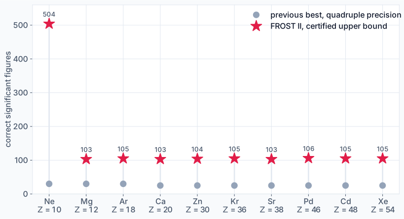
TLDR: In this post learn how to extend FROST from atoms with only \(s\) orbitals to every closed-shell atom from neon to xenon, and certify their Hartree–Fock energies as rigorous upper bounds: neon to 504 significant figures and the nine heavier atoms to 103–106, where the best previous values had 30 (up to argon) and 25. It takes three new ideas, one common wall for all orbitals, multiple shooting to tame inner shells that want to grow by \(10^{1701}\), and a homotopy that switches the electrons on slowly, and the certificate needs no logarithms at all, which I said last time it would.
This post is part of a series on Hartree-Fock theory:
- Restricted Hartree-Fock in 100 Lines: The original post; start here if new to HF
- Unrestricted Hartree-Fock in 100 Lines: Open shells and spin contamination
- The Integrals at the Heart of Hartree-Fock Theory: Every integral the basis-set approach needs, derived from scratch
- Hartree–Fock to 500 Significant Figures with FROST: We throw the basis set away, for helium and beryllium
- FROST II, Certified Hartree–Fock from Neon to Xenon: You are here, and we add \(p\) and \(d\) shells
The result (in hartrees)
Blue are the figures that were known before; red are new.
All ten atoms are in Part IV, along with every one of neon’s 504 figures.
Introduction, or how I was incorrect in the last post
The first FROST post ended with a list of what comes next, and the first item was \(p\) and \(d\) shells. I wrote that the solver would be unchanged, and that the certificate would need rigorous interval enclosures of logarithms instead of exact rationals. Both statements turned out to be wrong. The solver needed three new ideas before it could do a single heavy atom, and the certificate needed no logarithms at all, thanks to a choice of variable that Douglas Hartree made in 1928. Being wrong in this direction is my favourite kind of wrong.
Why bother? The answer is the same as last time: the method is the interesting part. A method that only works when every occupied orbital is an \(s\) orbital is a curiosity, as it covers helium, beryllium and not much else. Most of the periodic table has \(p\) and \(d\) shells, and for them the state of the art is Cinal’s pseudospectral method in quadruple precision, which in 2020 gave 25 significant figures for all 18 closed-shell atoms from helium to nobelium. Yamamoto and Hatano have since reported 30 figures for atoms up to argon, also in quadruple precision. No Hartree–Fock energy of a closed-shell atom beyond beryllium had been known to more than 30 figures.
Three things change when the occupied orbitals include \(p\) and \(d\) shells, and each one broke something:
- Multipoles. Exchange between orbitals of different angular momentum brings in the multipoles \(r_<^k/r_>^{k+1}\) with \(k\ge1\). Each needs its own potential, and krypton already has 47 of them
- Tails. Those multipoles hand every inner orbital the slowly decaying tail of the outermost one, so the separate walls of beryllium no longer work
- Stiffness. With one wall for everything, the krypton \(1s\) orbital has to be integrated out to 121 bohr, over which its growing mode rises by a factor of \(10^{1701}\)
The rest of the post is how FROST deals with each one.
What FROST takes from Hartree
In 1928, two years after Schrödinger’s equation, Douglas Hartree published “The Wave Mechanics of an Atom with a Non-Coulomb Central Field. Part I. Theory and Methods”, the paper that introduced the self-consistent field. This paper was the key inspiration behind FROST which keeps his formulation and replaces his arithmetic. The page numbers below are the journal’s; in Hartree’s notation the potential energy is \(-v\) and the energy is \(-\varepsilon/2\).
Solve the radial equation, not a basis expansion (§2, p. 92). Hartree writes the radial wave equation
\[P''+\big[2v-\varepsilon-l(l+1)/r^2\big]P = 0\]and says “This is the form in which the wave equation is used in the greater part of this paper.” Roothaan’s basis-set expansion came in 1951, and it was built for molecules, where the equations do not reduce to ODEs in one variable. For atoms Hartree’s route was never shown to be wrong; it was limited by hand arithmetic, which FROST removes.
The variable (§3, p. 95). This is the page that inspired my idea for FROST.
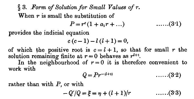 Hartree (1928), §3, p. 95: divide out the \(r^{l+1}\) behaviour at the nucleus and work with \(Q = Pr^{-(l+1)}\).
Near the nucleus the centrifugal term \(l(l+1)/r^2\) dominates the radial equation, and trying \(P = r^c\) gives Hartree’s indicial equation \(c(c-1) = l(l+1)\), with roots \(c = l+1\) and \(c = -l\). Only the first stays finite, so every orbital starts out as \(r^{l+1}\), and Hartree divides that factor out. Put \(P = r^{l+1}Q\) into his radial equation and multiply by \(r\), and you get
\[rQ''+2(l+1)Q' = -r(2v-\varepsilon)\,Q,\]which is FROST’s master equation \(ru''+2(L+1)u' = g\) with \(L = l\). FROST’s \(f\) is Hartree’s \(Q\). This one substitution does three jobs.
- The nucleus stops being singular. The equation for \(P\) has two terms that blow up at \(r = 0\), the Coulomb attraction \(2v \approx 2Z/r\) and the centrifugal term \(l(l+1)/r^2\), and \(r = 0\) is exactly where the integration has to start. In the equation for \(Q\) the centrifugal term has been absorbed into \(2(l+1)Q'\) and the Coulomb term appears as \(r\cdot2v \approx 2Z\), which is finite, so every coefficient is an ordinary power series. Substituting \(Q = \sum_k q_kr^k\) then gives each coefficient from the ones before it, \(q_{k+1} = g_k/[(k+1)(k+2l+2)]\), where \(g_k\) is the \(k\)-th coefficient of the right-hand side. That is what lets FROST start a Taylor series of hundreds of terms right at the nucleus
- The boundary condition at the nucleus takes care of itself. The unwanted solution \(r^{-l}\) becomes \(Q \propto r^{-(2l+1)}\), which is not a power series, so the recurrence cannot produce it. The only free number is \(q_0 = Q(0)\), which just sets the scale, and the first step of the recurrence gives \(q_1 = -Zq_0/(l+1)\), the cusp of the next paragraph. Nothing has to be imposed or fitted at \(r = 0\)
- Everything in the atom looks the same, and the certificate stays exact. FROST applies the same trick to the multipole potentials \(Y^k\), which start as \(r^{k+1}\), so a single recurrence integrates every orbital and every potential (§1). And because the \(r^{l+1}\) factors are carried explicitly, they cancel the \(1/r^{k+1}\) of the electron–electron interaction in the energy integrals, which keeps every integrand a polynomial and the certificate exact (Part III). With \(P\) the same integrals give logarithms
Hartree made the substitution so that a hand integration could start at the nucleus. It turns out to be what makes long Taylor series possible and what builds in the boundary condition and the cusp.
The cusp, and the degeneracy (§3, eq. 3·6, p. 95). Hartree starts each integration from a series at the nucleus, where \(v = N/r+v_0+\dots\) with \(N\) the atomic number, and finds that \(\xi = -Q'/Q\) equals \(N/(l+1)\) at \(r = 0\). That is \(Q'(0)/Q(0) = -Z/(l+1)\), the one-electron form of the cusp condition that FROST builds in, and that Kato later proved for many-electron wavefunctions. Hartree needed two terms of the series to start a hand integration; FROST uses hundreds, at every step. His second term contains the potential at the nucleus \(v_0\) and the energy \(\varepsilon\) only in the combination \(2v_0-\varepsilon\), which is the “cheeky degeneracy” \(\mu = \varepsilon - V_{\rm H}(0)\) of the first post, sitting in a 1928 equation.
Shooting (§2, p. 94, and §10, p. 108). Hartree’s method for the energy is to “integrate the equation outwards from \(P = 0\) at \(r = 0\), and inwards from \(P = 0\) at \(r = \infty\), and by trial find a value of \(\varepsilon\) for which these solutions meet at some convenient intermediate radius”. That is shooting with one matching point, two segments joined in the middle. The first FROST post shot outwards to a wall, and the multiple shooting of this post is Hartree’s matching with up to 125 segments instead of two.
Newton’s method (§4, p. 96, and §10). Hartree derives a “variation equation” for \(\partial P/\partial\varepsilon\) and uses it to predict how the mismatch between his two integrations changes with \(\varepsilon\), then interpolates: for a \(3d\) electron of rubidium a trial \(\varepsilon = 7.0\) gives 7.64. That is a Newton step with an analytic derivative. FROST’s Jacobian columns for the orbital energies are the same derivatives, formed by forward differences rather than by integrating his equation.
Growing modes (§10, p. 109). Hartree already knew the central difficulty which ended up being in both FROST papers. Beyond the outer turning point, he writes, “the integration outwards is highly unstable”, while integrating inwards is stable, so he started his inward integration at a finite radius outside the atom. FROST uses a hard wall there instead, because \(f(R) = 0\) makes the truncation variational, which the certificate needs, and then contains the growing modes with nested solves (the first post) or segments of bounded growth (this one).
The step size (§9, pp. 105–107). Hartree integrated with equal intervals and finite differences up to fourth order, doubling the interval as \(r\) grew, which the root test of FROST now does automatically at every step. And then, on p. 107, comes my favourite sentence in the paper:
“Doubtless it would be possible to derive formulae for integration over longer intervals with adequate accuracy, but the writer’s experience in other similar work is that simple formulae and a large number of intervals are much preferable to complicated formulae and a small number of intervals.”
FROST does exactly what Hartree called doubtless possible: Taylor series of order up to 873 and a handful of long steps, 41 of them to reach 109 bohr for helium. His reasons for not doing it were that every interval needed a slide-rule multiplication and had to be checked by hand, using the differences themselves. A computer and arbitrary-precision arithmetic remove both, and an independent run and an exact certificate take over the manual checking (aint nobody got time for that).
§1 of the same paper defines atomic units, with the unit of energy “twice the ionisation energy of the hydrogen atom”. That is the hartree, in which every FROST energy is quoted. In the outer region, where the field is Coulombic, Hartree used the exact Coulomb-field solutions (§§6–7), as the first FROST post did with Whittaker functions to predict the wall error.
What is not from Hartree (or what is new in the FROST method).
- Exchange, added by Fock and Slater in 1930. In 1928 Hartree also iterated the field until it reproduced itself, whereas FROST integrates Poisson’s equation alongside the orbitals, so there is no SCF loop at all
- Arbitrary precision and the exact certificate. The upper bound rests on the variational principle for a determinant, and has no 1928 counterpart
- The heavy-atom machinery of this post: the common tail and wall (Handy, Marron and Silverstone, 1969), multiple shooting with bounded growth, and the homotopy start
- The second job of \(Q\). Hartree introduced it to start an integration at the nucleus. In Part III it also keeps every integrand of the certificate a polynomial, thanks Hartree
Try the code yourself
FROST has outgrown a folder on this blog: it now has a C kernel, so the code lives in its own repository, github.com/adambaskerville/frost, where release v2.0 is the code of this post (v1.0 is the code of the first one). The orbitals of every run in this post, 1.4 GB compressed, are archived on Zenodo, doi:10.5281/zenodo.23884765, so you can check any of the bounds below with certify.py without repeating the run.
| file | what it does |
|---|---|
oracle_ns.py | the solver for any closed-shell atom |
taylor.c | its C kernel, compiled on first use |
certify.py | the exact certificate, for any \(l\) |
test_hf_taylor.py | end-to-end check (~11 s) |
paper2/run_all.sh | every run in this post |
You need Python 3 and gmpy2. The C kernel compiles against MPFR and GMP, which a conda environment provides; without them the solver falls back to pure Python, which works but is much slower. Times are for the 12 cores of an Apple M4 Pro laptop.
1
2
3
4
5
6
7
8
9
10
11
12
13
14
15
git clone https://github.com/adambaskerville/frost && cd frost
conda install -c conda-forge mpfr gmp   # for the C kernel
pip install -r requirements.txt

# neon to 100 digits (17 s), then its certified bound (16 s)
python oracle_ns.py --Z 10 --orbitals "1s 2s 2p" --digits 100 --out ne100.json
python certify.py ne100.json

# krypton to 30 digits (2.6 min), then its bound (2.8 min)
python oracle_ns.py --Z 36 --orbitals "1s 2s 2p 3s 3p 3d 4s 4p" \
    --digits 30 --out kr30.json
python certify.py kr30.json

# every run in this post (about 30 h)
paper2/run_all.sh runs && python paper2/make_paper2.py --extract runs
Birds-eye view
- Part I is what \(p\) and \(d\) shells change: one form for every equation, one wall for every orbital, and the stiffness that comes with it
- Part II is the numerics: Taylor recurrences, multiple shooting, Newton’s method, how to get started, and the C kernel
- Part III is the certificate for any angular momentum, and why I was wrong about the logarithms
- Part IV is the results: energies, the exchange-induced nodes of inner orbitals, and the cost
- Part V is the list of things that I messed up along the way, and Part VI the lessons and what comes next (again)
Part I: What \(p\) and \(d\) shells change
1. One form for every equation
Each orbital \(a\), with quantum numbers \((n_a, l_a)\), is doubly occupied in all \(2l_a+1\) magnetic sublevels, and its radial function \(P_a(r)\) behaves as \(r^{l_a+1}\) near the nucleus. Following Hartree, we divide this factor out and work with
\[f_a = P_a/r^{l_a+1},\]which is an ordinary power series at \(r=0\). In the first post \(f\) was the radial function \(R_{1s} = P/r\), which is the same thing for \(l=0\). This is Hartree’s \(Q\) from page 95 of his 1928 paper (shown above), which he introduced so that his hand integration could start at the nucleus; we will see in Part III that it also makes the certificate exact.
The electrons interact through one multipole potential for each pair of orbitals and each allowed \(k\),
\[Y^k_{ab}(r) = r\int_0^\infty P_a(s)P_b(s)\frac{r_<^k}{r_>^{k+1}}\,ds, \qquad k = |l_a-l_b|,\ |l_a-l_b|+2,\dots,\ l_a+l_b,\]and since these behave as \(r^{k+1}\) near the nucleus we likewise work with \(y^k_{ab} = Y^k_{ab}/r^{k+1}\). In these variables the closed-shell HF equations become
\[\begin{aligned} rf_a''+2(l_a+1)f_a' &= 2\Big[\Big(r\Big(2\sum_b(2l_b+1)y^0_{bb}-y^0_{aa}\Big)-Z-\varepsilon_ar\Big)f_a\\ &\qquad-\sum_{(b,k)\ne(a,0)}e^k_{ab}\,r^{k+1+l_b-l_a}\,y^k_{ab}f_b\Big],\\ ry^{k\,\prime\prime}_{ab}+2(k+1)y^{k\,\prime}_{ab} &= -(2k+1)\,r^{l_a+l_b+1-k}f_af_b, \end{aligned}\]with \(e^k_{ab} = (2l_b+1)\begin{pmatrix}l_a&k&l_b\\0&0&0\end{pmatrix}^2\) the usual angular factor. The first equation is the Fock equation: the Coulomb field of all the electrons less the self-exchange, the nucleus, the orbital energy, and then the rest of the exchange. The second is Poisson’s equation for each multipole. Because \(k\ge\vert l_a-l_b\vert\), every power of \(r\) in them is a non-negative integer, so nothing is singular.
The point of all this is that every equation has the same form (I think this might be the most significant thing in this whole method),
\[\boxed{\;ru''+2(L+1)u' = g\;}\]with \(L = l_a\) for an orbital and \(L = k\) for a potential, so a single Taylor recurrence integrates every unknown in the atom. At the nucleus the regular solution is fixed by \(u(0)\) alone, with slope \(u'(0) = g(0)/(2L+2)\). For an orbital that slope is \(f_a'(0) = -Zf_a(0)/(l_a+1)\), which is Kato’s cusp condition for any \(l\), built in exactly as before.
The bookkeeping grows quickly as krypton has 8 orbitals, 47 potentials, 36 pair products \(f_af_b\) and 73 exchange products \(y^k_{ab}f_b\), about a hundred convolutions per Taylor step. None of it is conceptually harder than helium, there is just more of it (reminds me when Dirac stated how the underlying physical laws of all of physics and chmistry are known, but the exact application leads to equations much too complicated to be soluble).
2. Every orbital gets the same tail
For beryllium each orbital had its own wall, placed where that orbital had decayed: the \(1s\) at 190 bohr and the \(2s\) at 744 for the 500-digit run. That worked because only the \(k = 0\) multipole appears between \(s\) orbitals, and far outside the atom it is proportional to the overlap of the two orbitals, which vanishes. Exchange then has no long-range part, and each orbital decays at its own rate \(e^{-\kappa_ar}\), with \(\kappa_a = \sqrt{-2\varepsilon_a}\).
With \(k\ge1\) that argument fails. Far outside the density \(Y^k_{ab}\to m^k_{ab}/r^k\), where \(m^k_{ab} = \int s^kP_aP_b\,ds\) is the multipole moment of the pair, and it is generally not zero. The exchange term in the equation for orbital \(a\) then behaves as \(m^k_{ab}\,r^{-k-1}P_b(r)\), so the tail of orbital \(b\) drives orbital \(a\). If \(b\) is the outermost orbital, its tail decays more slowly than \(a\)’s own and wins. Through chains of such couplings every orbital inherits the decay of the highest occupied orbital, as Handy, Marron and Silverstone showed in 1969.
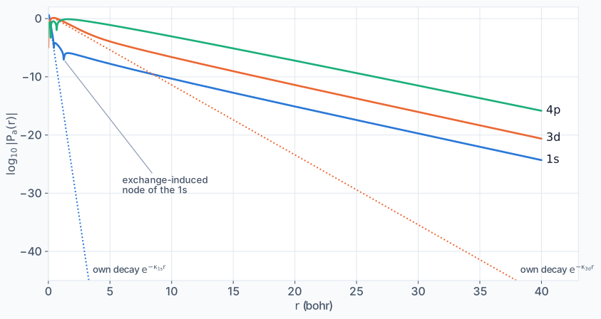 Krypton’s \(1s\), \(3d\) and \(4p\) orbitals from the certified 100-digit run. Dotted: the decay \(e^{-\kappa_ar}\) that the \(1s\) and \(3d\) would have on their own, drawn from each maximum. Instead both fall off in parallel with the outermost \(4p\). The dip at 1.26 bohr is one of the \(1s\) orbital’s two exchange-induced nodes (Part IV).
The size of the effect is significant as at 10 bohr the krypton \(1s\) is \(10^{-11}\) of its maximum, where its own decay would have taken it to \(10^{-140}\): the induced tail is 129 orders of magnitude larger than the tail you would naively expect. A wall at the \(1s\) orbital’s own decay length would cut off a tail that is really there. I found this the hard way in neon, where moving the \(1s\) wall changed the residuals of the other equations at the \(10^{-6}\) level, which rules out separate walls at any serious accuracy.
So FROST II uses one common wall \(R\) for all orbitals, with
\[f_a(R) = 0, \qquad Ry^0_{aa}(R) = 1, \qquad Ry^{k\,\prime}_{ab}(R)+(2k+1)\,y^k_{ab}(R) = 0 .\]The first is the wall, the second is normalisation (since \(Y^0_{aa}(R) = \int_0^RP_a^2\,dr\), the same trick as in the first post), and the third holds exactly outside the density, where \(y^k_{ab}\propto r^{-(2k+1)}\). The wall error still falls as \(e^{-2\kappa R}\), now with \(\kappa\) that of the outermost orbital, so for \(D\) digits \(R = (D+8)\ln10/(2\kappa)\) as before.
The common wall brings a bonus. The orbitals of one symmetry are now eigenfunctions of a single self-adjoint Fock operator on \([0,R]\), so they are exactly orthogonal. The orthogonality saga that cost the most time in the beryllium work, with its Lagrange multipliers and a \(2s\) “normalisation” of 1245, simply disappears.
Main lesson I learned. The hardest part of the last project went away once the physics forced a different boundary condition. If a constraint is fighting you, check whether you have set the problem up the way nature wants it.
3. Stiffness, or krypton’s \(10^{1701}\)
The common wall has a price. Away from the nucleus each orbital equation has a decaying solution \(e^{-\kappa_ar}\) and a growing one \(e^{+\kappa_ar}\), and in the first post we saw that a wrong orbital energy lets the growing one take over. With one wall far out, the inner orbitals must be integrated over the whole range, and for krypton, with \(\kappa_{1s} = 32.25\) and \(R = 121.44\) bohr,
\[e^{\kappa_{1s}R} = 10^{1701}.\]Single shooting from the nucleus amplifies any error in the starting values by this factor, so it would need about 1,700 digits of working precision on top of the 100 we want. Beryllium’s nested scalar shooting, which kept the growing modes out of the outer problem, has no answer to this either: the growth is not a conditioning problem that a cleverer solve order can hide, it is the size of the numbers themselves.
Part II: The numerics
The equations of Part I form a nonlinear eigenvalue problem in which the orbitals, their potentials and the orbital energies are all coupled. FROST II solves it in four layers: Taylor series integrate the equations step by step, multiple shooting cuts \([0,R]\) into segments so that the inner orbitals’ growing modes never swamp the precision, Newton’s method solves the resulting algebraic equations, and a homotopy followed by a sequence of growing walls gives us our starting point.
4. Taylor recurrences for any \(L\)
Substituting \(u = \sum_ku_k(r-r_0)^k\) into our laster equation, \(ru''+2(L+1)u' = g\) gives, about \(r_0>0\),
\[u_{k+2} = \frac{g_k-(k+1)(k+2L+2)\,u_{k+1}}{r_0(k+1)(k+2)},\]and at the nucleus \(u_{k+1} = g_k/[(k+1)(k+2L+2)]\). For \(L = 0\) these are exactly the recurrences of the first post. The right-hand sides are products of orbitals and potentials, so their coefficients \(g_k\) are Cauchy products again, and as before each step covers a fraction \(c\) of the radius of convergence that the root test reads off the last few coefficients. One small change: the root test now uses \(\max(\vert f_0\vert,\vert f_1\vert)\) as its scale rather than \(\vert f_0\vert\), because an expansion point that lands exactly on a node of the \(2s\) would otherwise fake a tiny radius.
One subtlety matters a great deal for heavy atoms, and it took me longer to find than I would like to admit. The root test only sees the solution, and far out the solution is every orbital riding the slow common tail, so near the wall it happily allows a single Taylor step across a whole two-bohr segment. Newton’s method, however, does not only work with the solution. Its corrections and Jacobian columns are made of each orbital’s own fast modes \(e^{\pm\kappa_ar}\), and for the zinc \(1s\) one such step spanned \(\kappa_{1s}h\approx53\), which at order 140 resolves those modes to only 15–20 digits. That is enough to make Newton’s method fail at 100 digits.
The fix comes straight out of the first post. There, the radius-of-convergence figure showed that far from the nucleus a finite-order root test sees the coefficients \(\kappa^k/k!\) of the exponential first, and \((k!)^{1/k}/\kappa\approx k/(e\kappa)\). So at order \(p\) the series of \(e^{\kappa r}\) behaves as if its radius were \(p/(e\kappa)\), and FROST II caps every step at \(c\) times that, using the largest \(\kappa_a\):
1
2
3
4
5
6
7
def stiff_cap(eps, c, p):
    """Cap the step at c p / (e kappa_max), in 2^-16 units: the modes
    exp(+-kappa r) that Newton works with have that order-p radius."""
    m = float(min(eps))
    if m >= 0:
        return math.inf
    return math.floor(c * p / (math.e * math.sqrt(-2 * m)) * 65536)
The cap only binds where the fast modes would otherwise be under-resolved, and it leaves the energies of the light atoms unchanged to every printed digit.
5. Multiple shooting
Multiple shooting is an old idea from boundary-value problems: rather than integrate from one end and hope, cut the interval into segments \(0 = r_0<r_1<\dots<r_J = R\) and integrate each one independently from its own starting state. The unknowns are now
- the start values \(f_a(0)\) and \(y^k_{ab}(0)\),
- the full state \((f_a, f_a', y^k_{ab}, y^{k\,\prime}_{ab})\) at every interior knot,
- and the orbital energies \(\varepsilon_a\),
and the equations say that the state is continuous at every interior knot and that the wall conditions hold at \(R\). For krypton that is 110 unknowns per knot and 67 segments, 7,323 unknowns in all, against two for helium.
The segments are chosen so that no growing mode rises, relative to the bulk density \(e^{-\kappa r}\), by more than a factor \(10^g\) across one. An error in a segment’s starting state is then amplified by at most \(10^g\), the linear solve loses at most another \(g\) digits, and for \(d\) target digits we work with \(d+2g+40\) digits. That margin depends on \(g\) and not on how stiff the atom is. A stiffer atom simply gets more segments; xenon has 103 and cadmium 125. The \(10^{1701}\) never appears in the arithmetic.
An inner orbital only needs to shorten the segments where it is large. Beyond its own radius \(n_i/\kappa_i\) it has already fallen below the bulk, and it may grow back by as much as it has fallen, but by no more than about \(10^4\), the level of its induced tail:
1
2
3
4
5
6
7
8
9
10
def knots(R, kap, ns, g):
    """No orbital's growing mode may outgrow the bulk by more than 10^g
    per segment. kap: each orbital's kappa; ns: its n."""
    kt, ks = min(kap), [0.0]
    while ks[-1] < R:
        r = ks[-1]
        L = min((g * LN10 + min((k - kt) * max(r - n / k, 0), 4 * LN10))
                / (k + kt) for k, n in zip(kap, ns))
        ks.append(min(max(up(r + L), r + 1 / 64), R))
    return ks
(Simplified from oracle_ns.py; up rounds up to the \(1/64\) grid so that every knot is an exact dyadic rational, which the certificate needs.)
6. Newton’s method, done cheaply
The system is solved by a chord Newton iteration (which I was not aware of but came across in reading around Newton solvers for FROST, so I learned this on the job), which keeps one Jacobian and refreshes it only when a step fails to shrink the correction threefold. The Jacobian is formed by forward differences, with all its columns computed in one parallel batch. Here the segments pay off a second time: a column for a knot state only needs one segment to be integrated again, while a column for an \(\varepsilon_a\) needs all of them.
The Jacobian has a lovely structure, block bidiagonal with \(-I\) coupling each segment to the next knot, plus dense columns for the orbital energies. A sparse LU with row equilibration and partial pivoting keeps the fill inside the band, so the linear algebra costs well under the integrations.
The cheapest trick is in the precision. A chord iteration converges as long as its Jacobian is accurate enough to contract, so during the wall continuation (§7) FROST builds and factors the Jacobian at only about \(4g+30\) digits, with a matching lower Taylor order, while the residuals are always evaluated at full precision. The converged solution is therefore unchanged, because accuracy comes from the residual and not from the Jacobian, and if a cheap Jacobian fails it is rebuilt at full precision. The result of this is that it roughly halved the run times, lovely.
7. Getting started: switch the electrons on slowly
Newton’s method needs a starting point close to the ground state, and the HF equations of a heavy atom have plenty of other solutions, including ones in which the wall squeezes an orbital to positive energy. A screened hydrogenic guess, which was fine for helium, is nowhere near good enough for xenon.
So FROST II starts from a problem which it can solve exactly, multiply every electron–electron term in the Fock equation by \(t\) (a trick I learned in my PhD). At \(t = 0\) the electrons do not see each other, the orbitals are hydrogenic and known in closed form, and the solution is then followed in small steps to \(t = 1\). Each step changes the potentials by a finite amount, which a segment amplifies by \(10^g\), so the homotopy keeps \(g = 1\) and a modest 10-digit target. The step in \(t\) starts at \(1/32\), grows after an easy step and halves after a failure. Meanwhile the wall moves with the orbitals, at \(R = \max_a(2n_a+6)/\kappa_a(t)\), where every hydrogenic \(r^{n-1}e^{-\kappa r}\) has fallen to about \(10^{-3}\) of its peak, so that no orbital gets squeezed (see Part V for how I learned that).
The second stage moves the wall out to its final value, as in the first post, with each stage targeting the digits its wall can deliver, \(\min(D, 2\kappa R/\ln10)+10\). Moving the wall changes the solution only by about \(e^{-\kappa R}\) near the old wall, so these stages can afford long segments, with \(g\) up to 30, and the wall grows by a factor between 1.2 and 2 per stage depending on how easy the last one was. The guess on the new knots is the previous solution integrated out to them and continued beyond the old wall with each orbital’s own logarithmic derivative and each potential’s multipole tail.
8. A little C
The orchestration (homotopy, continuation, Newton’s method and knot placement) is a few hundred lines of Python with gmpy2, as before. I love Python but profiling said 93% of the time went into the Cauchy products of the Taylor series (ugh), so I moved the integration of a segment and the sparse LU moved into a small C library on MPFR and GMP, called through ctypes (also, controversial opinion, C is superior to C++. I will gladly die on this hill). It is compiled on first use, the pure-Python integration stays as a fallback, and the test checks one against the other (because you always should).
A Cauchy product coefficient is a sum \(\sum_iu_iv_{k-i}\), and the obvious multiply-and-add loop rounds \(2k+1\) times. Instead, each product of two MPFR numbers is formed exactly as an integer mantissa and added into a wide fixed-point accumulator, and the sum is rounded once at the end, an idea that I learned from (I think) Kulisch. It is more accurate, and it is also 1.8 to 2.4 times faster at 170–400 bits, because exact limb multiplications are cheaper than rounded ones. Segments and Jacobian columns are spread over a pool of processes, one per core.
Part III: The certificate, and why I was wrong (no surprises there)
The certificate is the same idea as before: a separate program reads the solver’s orbitals, which are piecewise polynomials with exact dyadic coefficients, imposes continuity and the wall exactly, and evaluates the energy in exact rational arithmetic. By the variational principle the result is a rigorous upper bound, with no rounding anywhere.
For more than one symmetry it uses the closed-shell determinant energy, which, like the beryllium formula of the first post, depends only on the space the orbitals span and never assumes they are orthonormal:
\[\begin{aligned} E = {}&2\sum_l(2l+1)\sum_{i,j\in l}D_{ij}h_{ij}\\ &+\sum_{l,l'}(2l+1)(2l'+1)\sum_{\substack{i,j\in l\\m,o\in l'}}D_{ij}D_{mo}\Big[2R^0(ij,mo)-\sum_k\begin{pmatrix}l&k&l'\\0&0&0\end{pmatrix}^2R^k(im,jo)\Big], \end{aligned}\]with \(D = S^{-1}\) inverted exactly in each block of equal \(l\), and the Slater integrals
\[R^k(ij,mo) = \iint P_iP_j(r)\,P_mP_o(s)\,\frac{r_<^k}{r_>^{k+1}}\,dr\,ds .\]The squared \(3j\) symbols are rational numbers, so they are carried exactly. The one-electron integrals are easy. In terms of \(f\), and after integrating the centrifugal term by parts,
\[T_{ij} = \frac12\int_0^Rr^{2l+2}f_i'f_j'\,dr,\qquad V_{ij} = -Z\int_0^Rr^{2l+1}f_if_j\,dr,\]because the terms in \(r^{2l}f_if_j\) cancel, \(-(l+1)(2l+1)+(l+1)^2+l(l+1) = 0\), which is the sort of cancellation that makes my day.
Now the part I got wrong. In the first post I said that the multipole factor \(r_>^{-k-1}\) integrated over a polynomial element gives logarithms of knot ratios, so the certificate would need interval enclosures of logarithms. That is true if you work with \(P\). But split each Slater integral into its two orderings, \(R^k(q,p) = C^k(q,p)+C^k(p,q)\), with
\[C^k(q,p) = \int_0^Rr^{\,l_q+1-k}f_if_j(r)\,Q^k_p(r)\,dr,\qquad Q^k_p(r) = \int_0^rs^{\,l_p+k+2}f_mf_o\,ds,\]where \(q = (ij)\), \(p = (mo)\) and \(l_q = l_i+l_j\). The factor \(r^{-k-1}\) has combined with \(P_iP_j = r^{l_q+2}f_if_j\) into \(r^{l_q+1-k}\), and the triangle rule of angular momentum says \(k\le l_i+l_j\). So the power is never negative, every integrand is a polynomial, and every integral is an exact rational. With \(P\) the same integrands contain negative powers of \(r\), which is where my logarithm idea came from.
So Hartree’s \(Q = Pr^{-(l+1)}\), introduced in 1928 to make it easier to start a numerical integration at the nucleus, is what turns the energy of a heavy atom into the method developed here 98 years later, rather delightful if I do say.
Two practical notes. The inner integral \(Q^k_p\) is carried across the polynomial pieces as an exact antiderivative, and apart from it the pieces are independent, so the certificate now processes them in parallel: each piece returns its own contributions, and a prefix sum over the pieces supplies the running integrals. The parallel program returns the identical rational, five to ten times faster. And for \(s\) shells alone it returns the same rational as the certificate of the first post, bit for bit.
Part IV: Results
Energies
Every atom has a certified run A and an independent run B, which targets 10 more digits with a larger wall, a different step fraction (\(c = 0.25\) against 0.15) and fewer guard digits, and so a different mesh, order, knots and precision. Run B’s own wall error is about \(10^{-10}\) of run A’s, so the distance between run A’s certified bound and run B is the distance of the bound from the HF limit, and that is how the number of correct figures below is counted. Neon targets 500 digits; the others target 100, for reasons of patience (see the cost below). Walls are in bohr, “s.f.” is the number of correct significant figures and “prev.” the best previous number.
| atom | \(E_{\rm HF}\le\) (hartree) | wall | segments | s.f. | prev. |
|---|---|---|---|---|---|
| Ne (\(Z\) = 10) | −128.547098109382042376475781341… | 448.47 | 54 | 504 | 30 |
| Mg (12) | −199.614636424506710474741636103… | 174.78 | 31 | 103 | 30 |
| Ar (18) | −526.817512802723355018766093533… | 114.38 | 31 | 105 | 30 |
| Ca (20) | −676.758185924513454948055751766… | 198.84 | 59 | 103 | 25 |
| Zn (30) | −1777.84811619136106977844250329… | 162.58 | 71 | 104 | 25 |
| Kr (36) | −2752.05497734557645439444913823… | 121.44 | 67 | 105 | 25 |
| Sr (38) | −3131.54568643855718443412415394… | 208.14 | 112 | 103 | 25 |
| Pd (46) | −4937.92102407010157293228980380… | 151.69 | 99 | 106 | 25 |
| Cd (48) | −5465.13314253008643367281863127… | 170.84 | 125 | 105 | 25 |
| Xe (54) | −7232.13836387184088820928921655… | 130.03 | 103 | 105 | 25 |
Correct significant figures of each certified bound (red) against the previous best (grey), Yamamoto and Hatano up to argon and Cinal beyond, both in quadruple precision. Neon targeted 500 digits, the others 100.
Here are all 504 correct figures of neon, from the 500-digit run with a wall at 448 bohr, Taylor order 626 and 2,026 bits of working precision:
Three checks are independent of the A/B comparison:
- Published values. All 25 digits of Cinal’s quadruple-precision energies agree with ours after rounding, for all ten atoms, and so do his 22–25-digit energies of the highest occupied orbital
- Orthogonality. The canonical orbitals of each symmetry are orthogonal to the working precision, for example \(\vert S_{ij}\vert\le8\times10^{-114}\) for krypton, as the common wall says they must be. The certificate does not rely on this
- Upper bounds. Every certified bound lies above the energy of the more accurate run B, as it must
Exchange-induced nodes
The induced tails of §2 have a strange consequence where an inner orbital’s own part has decayed to the size of its induced tail, the two can cancel, and the orbital picks up a node that the hydrogenic orbital does not have. I thought a \(1s\) orbital with a node was a bug, and in a basis-set calculation it is hard to tell a real node from the spurious wiggles of a finite basis. It turns out that such nodes have been reported for the \(1s\) orbitals of argon, zinc and krypton and the \(2s\) of krypton, and traced to exchange by Hatano, Tatewaki and Yamamoto.
Interestingly, in FROST they come out of the solution with no special treatment. Bisection on the certified piecewise polynomials locates each sign change to 100 decimal places, and runs A and B agree on almost all of them to every figure of the bisection. The pattern is exactly what §2 predicts:
- Magnesium, whose orbitals are all \(s\) orbitals, has none, as the \(k = 0\) argument requires
- Argon has one, in the \(1s\)
- Calcium and zinc have them in the \(1s\) and \(2p\); krypton and palladium also in the \(2s\); strontium and cadmium also in the \(3p\) and \(3d\); and xenon also in the \(3s\)
For krypton, where Cinal gives ten figures (all of which agree):
| orbital | node (bohr) |
|---|---|
| \(1s\) | 0.448341935663648833694790412998… |
| \(1s\) | 1.25556571438079398219168513125… |
| \(2s\) | 1.50628509424546649132420533515… |
| \(2p\) | 2.23877072824654668461219855581… |
The krypton \(1s\) changes sign twice, at 0.45 and 1.26 bohr, where it is 5–7 orders of magnitude below its maximum, which is the dip in the tails figure. The \(1s\) orbitals of palladium and xenon manage three. Because the error of a FROST orbital is the wall’s, and that is exponentially small in the core, the nodes are known to about as many figures as the energies. The full list, 38 nodes in all, is in the paper.
Cost
All runs were made one at a time on the 12 cores of an Apple M4 Pro laptop.
| atom | run A | run B | certificate |
|---|---|---|---|
| Ne (500 digits) | 26 min | 41 min | 17 min |
| Mg | 86 s | 4 min | 3 min |
| Ar | 13 min | 9 min | 6 min |
| Ca | 7 min | 15 min | 11 min |
| Zn | 24 min | 51 min | 16 min |
| Kr | 37 min | 43 min | 25 min |
| Sr | 1.8 h | 1.5 h | 71 min |
| Pd | 1.9 h | 1.6 h | 54 min |
| Cd | 1.6 h | 2.1 h | 1.6 h |
| Xe | 3.9 h | 3.2 h | 2.1 h |
The cost is dominated by the Jacobians. Each costs as much as \(m+n\) integrations of the full range, one per unknown at a knot plus one per orbital energy (118 for krypton), albeit in lower precision, while a Newton iteration costs one. Heavier atoms cost more because they have more potentials, roughly the square of the number of orbitals, and more segments. Nothing in the method stops xenon going to 500 digits; it would just take a lot longer.
Part V: Things that I broke along the way
FROST II broke more often than FROST, and most of the failures were interesting.
- Separate walls. My first attempt kept beryllium’s one wall per orbital. Neon’s residuals moved at \(10^{-6}\) when the \(1s\) wall moved, which is how I met the induced tails of §2
- A precision frozen into a constant. The \(3j\) coefficients were built as MPFR numbers inside the setup function, which ran during the 52-digit homotopy, so every later stage used exchange coefficients good to 52 digits. Two 100-digit neon runs agreed to only 87.6 figures, and the virial gap, \(E+T\), sat stubbornly at \(10^{-52}\). The fix was to keep the squared \(3j\) symbols as exact rationals
- The context manager lied to me.
gmpy2.local_contextrestores a copy of the context on exit, so a handle to the old context held elsewhere quietly detached, and every later stage ran at the old precision. Newton’s method floored at ten times its tolerance with no error anywhere. The fix was to save and restore the precision by hand, and the code now carries a comment warning my future self because I can guarantee I will forget - A quadratic parser.
mpfr_strtofrcallsstrlenon its whole argument, so parsing a long buffer of numbers one at a time was quadratic: the LU input took 21 s to read. Copying each token first fixed it - A \(5s\) orbital in a box. The homotopy wall started out at \(8/\kappa\) of the outermost orbital, which is fine up to \(n = 4\). A hydrogenic \(5s\) is still about 30% of its peak there, so the wall squeezed it to positive energy, and the xenon run sat on this box state for six hours. The wall is now \(\max_a(2n_a+6)/\kappa_a\), and any step that ends with an \(\varepsilon_a\ge0\) is rejected
- A shortcut that found the wrong atom. To save time I tried freezing the knots during the homotopy and reusing the LU. Krypton drifted onto a different branch of solutions and converged happily to an energy correct to 2.5 figures. Instantly reverted
- Cheap Jacobians in the homotopy. The low-precision Jacobian of §6 also broke the homotopy, with a singular Jacobian for cadmium and a NaN step for xenon. The homotopy now uses full-precision Jacobians, and a cheap Jacobian that is singular or gives a non-finite residual is rebuilt at full precision
- A 0.2-bohr sliver. Argon’s 100-digit run failed on a final wall stage only 0.2 bohr long. A stage now goes straight to the final wall when it is close
- The step that took most time. Calcium, zinc and krypton all failed at 100 digits in the final stages, with Newton diverging or producing non-finite residuals. The obvious suspect was the sparse LU. I saved the failing stage to disk and replayed it, and the LU was innocent: its backward error was \(10^{-137}\), and the step it gave was identical at one, two and four times the precision. The real culprit was the root test of §4 allowing one Taylor step across a whole segment. With the step cap, the replayed residual went from \(6\times10^{-34}\) to \(10^{-71}\) in a single Newton step, and all ten atoms then ran with no failures
Lesson. Two of these failures were the arithmetic silently running at a lower precision than I asked for, and the virial gap caught both.
For anyone wanting to calculate anything to high precision, this message is very, very important; watch an invariant whose value you know, and when something fails in a long run, save the failing state and replay it with more precision before you guess what is wrong; I would still be rewriting the LU otherwise.
One of the easiest mistakes with high precision calculations, from extensive experience, is that a single operation can crash your precision back to double because precision was not maintained correctly at every stage. Check that every step you implement received the memo about the precision you want to run at.
Part VI: What might trasnfer to other fields
Lessons
- Let the physics choose the boundary conditions. The induced tails force one wall, and one wall gives exact orthogonality for free. The constraint I spent the most time on in the first post was a symptom of the wrong setup
- Stiffness is a precision problem only if you shoot once. Multiple shooting turns a growth of \(10^{1701}\) into more segments, with a precision margin that depends on the segment growth, not the atom
- A chord iteration only needs a Jacobian that contracts. Build it cheaply, evaluate the residual exactly, and the answer is as good as the residual
- Start from a problem you can solve. Switching the electron–electron interaction on from zero turns “find the ground state of xenon” into a sequence of small, safe steps from hydrogen-like orbitals
- The right variable can turn an approximation into a proof. Dividing out \(r^{l+1}\) keeps every certificate integrand polynomial; with \(P\) it would have needed logarithms
- An adaptive step is only as good as what it can see. The root test saw the solution and not the modes Newton works with. If your step control is driven by one quantity, check that nothing else needs resolving
- Replay failures; do not guess. Saving and replaying the failing stage cleared the LU and found the real bug
- Exact dot products are cheaper than I thought. Forming products exactly and rounding once was both more accurate and twice as fast
What next
- \(f\) shells. The remaining closed-shell atoms of Cinal’s set, barium, ytterbium, mercury, radon, radium and nobelium, add an \(f\) shell or more electrons. Neither changes the formulation: the multipoles go up to \(k = 6\) and the certificate is unchanged. The cost per digit grows with the number of potentials and with the stiffness through the number of segments, so these are patience rather than ideas
- Open shells need the restricted open-shell energy expression with its additional couplings
- Diatomic molecules. The radial ODEs become PDEs in prolate spheroidal coordinates, and the method would need a two-dimensional analogue of the Taylor segments. I have no idea yet how to do that, which is exactly why it is interesting
- A lower bound. As before, the distance to the limit comes from an independent run and the exponential decay of the wall error, not a theorem. A certified lower bound for a nonlinear eigenproblem at this precision is still an open problem, so answers on a postcard again please
References
- D. R. Hartree, “The wave mechanics of an atom with a non-Coulomb central field. Part I. Theory and methods”, Proc. Camb. Phil. Soc. 24, 89 (1928).
- V. Fock, Z. Phys. 61, 126 (1930).
- J. C. Slater, Phys. Rev. 35, 210 (1930).
- C. C. J. Roothaan, “New developments in molecular orbital theory”, Rev. Mod. Phys. 23, 69 (1951).
- N. C. Handy, M. T. Marron and H. J. Silverstone, “Long-range behavior of Hartree-Fock orbitals”, Phys. Rev. 180, 45 (1969).
- T. Kato, “On the eigenfunctions of many-particle systems in quantum mechanics”, Commun. Pure Appl. Math. 10, 151 (1957).
- E. Clementi and C. Roetti, At. Data Nucl. Data Tables 14, 177 (1974).
- C. Froese Fischer, The Hartree–Fock Method for Atoms: A Numerical Approach (Wiley, 1977).
- G. S. Handler, D. W. Smith and H. J. Silverstone, J. Chem. Phys. 73, 3936 (1980).
- T. Ishida and K. Ohno, Theor. Chim. Acta 81, 355 (1992).
- U. M. Ascher, R. M. M. Mattheij and R. D. Russell, Numerical Solution of Boundary Value Problems for Ordinary Differential Equations (SIAM, 1995).
- C. T. Kelley, Iterative Methods for Linear and Nonlinear Equations (SIAM, 1995).
- L. Fousse, G. Hanrot, V. Lefèvre, P. Pélissier and P. Zimmermann, “MPFR: A multiple-precision binary floating-point library with correct rounding”, ACM Trans. Math. Softw. 33, 13 (2007).
- S. L. Saito, At. Data Nucl. Data Tables 95, 836 (2009).
- J. Kobus, Comput. Phys. Commun. 184, 799 (2013).
- U. Kulisch, Computer Arithmetic and Validity: Theory, Implementation, and Applications, 2nd ed. (de Gruyter, 2013).
- N. Takeda, Y. Hatano, S. Yamamoto and H. Tatewaki, Comput. Theor. Chem. 1045, 99 (2014).
- M. P. A. Mendez, D. M. Mitnik and J. E. Miraglia, Int. J. Quantum Chem. 116, 1882 (2016).
- S. Lehtola, Int. J. Quantum Chem. 119, e25945 (2019).
- M. Cinal, J. Math. Chem. 58, 1571 (2020).
- Y. Hatano, H. Tatewaki and S. Yamamoto, Comput. Theor. Chem. 1204, 113400 (2021).
- J. Kobus and S. Lehtola, Comput. Phys. Commun. 311, 109576 (2025).
- S. Yamamoto and Y. Hatano, J. Math. Chem. 64, 42 (2026).
- The code: github.com/adambaskerville/frost, release v2.0; the orbitals: doi:10.5281/zenodo.23884765.
- My earlier posts: “Hartree–Fock to 500 Significant Figures with FROST” and “Helium to 60 Significant Figures with FLAKE”.