T>T: Do Four-Body Perimetric Coordinates Exist?

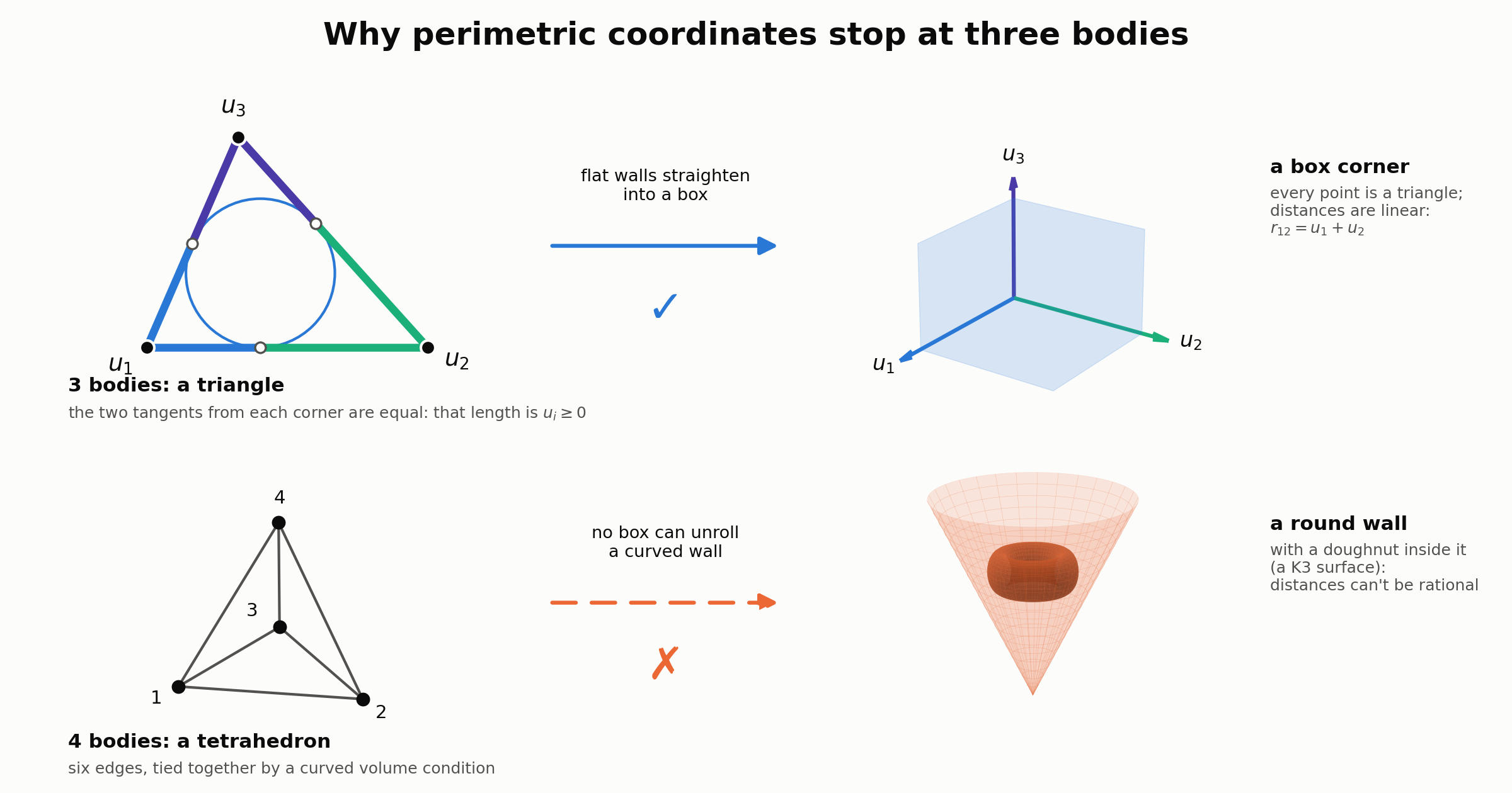
Try the code yourself!

Click the following button to launch an ipython notebook on Google Colab which implements every check in this post:

All of the code lives in FourBodyPerimetricCode/: four_body_perimetric.py is the walk-through you see below, checks.py is the full battery of assertions behind every claim, he_graded.py is the helium experiment from the second half of the post, and make_diagrams.py, make_figures.py and make_headliner.py draw every picture.

The problem

If you have read my Pekeris post you will know that I have a soft spot for perimetric coordinates. They are the trick that made Pekeris’ 1958 helium calculation possible: three numbers that range independently over $[0,\infty)$, in which the awkward triangle-shaped domain of the three-body problem becomes a simple box, the Schrödinger equation becomes a sparse recurrence, and a 1950s computer can solve helium.

The obvious next question which many have asked, myself included for many years, is:

what about four particles?

Lithium, the positronium molecule, H$_2$ with moving nuclei, the hydrogen molecular ion with a muon… all of these are four-body problems. If someone handed us six “perimetric coordinates” for four particles that did for the tetrahedron what Pekeris’ did for the triangle, a lot of very expensive calculations would suddenly become cheaper.

I attempted to derive four particle perimetric coordinates during my PhD but ended up with nothing, however I started to think about them again recently and decided to refresh my memory as to what the literature shows. However when I went looking the literature was a mess; there were claims in both directions and nobody seemed to agree on what the question even was:

• In 1966 Rasiel and Karl attempted a construction and conjectured that no such coordinates exist
• White replied the same year, and in 1967 Jug published a short paper whose abstract says four-particle perimetric coordinates do not exist
• Wang (1967) proposed nonlinear coordinates that range independently over $[0,\infty)$, and Carter (1968) proposed “normal” coordinates
• In 2006 Frolov published “Four-body perimetric coordinates”, claiming six coordinates that “describe all possible configurations in an arbitrary four-body system”
• In 2014 a master’s thesis by Kreuter pointed out that Frolov’s constraints are necessary but not sufficient, i.e. “this paper is in error”
• In 2016 Frolov himself wrote that it is “impossible to define six perimetric coordinates (for four-body systems) which have the same properties” as the three-body ones

So which is it? I wanted to (attempt) to settle it once and for all, or at least get as close to “once and for all” as a spare-time project allows. This post is a timeline of how that went, including the dead ends, because the dead ends turned out to be where most of my understanding came from.

TLDR: not to get too philosophical but it depends on what you mean by “exist”, and once you say precisely what you mean, every version of the question has a definite answer:

• Coordinates that are linear in the distances: no
• Coordinates that are smooth right up to the boundary like Pekeris’: no
• Independent coordinates where the squared distances are polynomials: yes, they exist
• Independent coordinates where the distances themselves are rational (e.g. polynomial) functions, which is the version that would actually be useful: no, and the reason is that a K3 surface is hiding inside the geometry of a flat tetrahedron. On top of that, any Pekeris-style sparse method for four-body Coulomb problems is ruled out by a Galois-theory argument that I could watch fail in a helium calculation

What perimetric coordinates actually do

For three particles the three distances $r_{12}, r_{13}, r_{23}$ cannot be anything you like. They have to satisfy the triangle inequalities in order to correctly map the space,

\[r_{12} \le r_{13} + r_{23},\qquad r_{13} \le r_{12}+r_{23},\qquad r_{23}\le r_{12}+r_{13}.\]

Perimetric coordinates are the three “slacks” in those inequalities:

\[u_1 = \tfrac12(r_{12}+r_{13}-r_{23}),\qquad u_2 = \tfrac12(r_{12}+r_{23}-r_{13}),\qquad u_3 = \tfrac12(r_{13}+r_{23}-r_{12}).\]

Geometrically they are the lengths of the tangents from each vertex of the triangle to its inscribed circle. Each inequality becomes “$u_i \ge 0$”, and the domain of allowed triangles becomes the positive octant $[0,\infty)^3$, every point of the octant is a genuine triangle, and the distances are linear in the new coordinates, $r_{12} = u_1+u_2$ and so on.

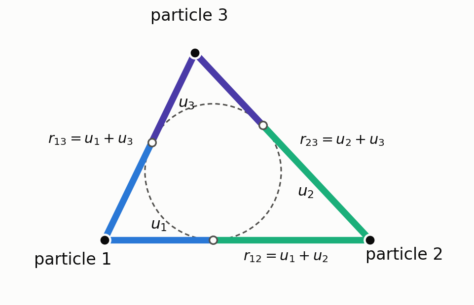
Each side of the triangle is cut in two by the point where the incircle touches it, and the two pieces belong to the two vertices at either end. Every vertex owns two equal tangent pieces (same colour above), so three numbers $u_1, u_2, u_3$ describe the whole triangle, and you can shrink any one of them to zero without the others caring.

That last property is what Pekeris really exploited, becayse the distances are linear, the Coulomb terms $1/r_{ij}$ can be cleared by multiplying through by a polynomial, the exponential $e^{-\alpha r}$ factorises, and the whole problem collapses into a recurrence with a fixed number of terms per row.

So when we ask ourselves “do four-body perimetric coordinates exist?”, there are really several properties being wished for at once:

1. six coordinates that range independently (the domain is a box),
2. every point of the box is a genuine configuration, and every configuration is reached,
3. the distances are simple (linear, or at least polynomial) functions of the coordinates,
4. and ideally the whole thing is smooth right up to the edges, like Pekeris’ map.

Keep that list in mind, because the conclusion is that you can have some of these but not all of them.

The four-body domain

Four particles have six distances, $r_{12}, r_{13}, r_{14}, r_{23}, r_{24}, r_{34}$: the six edges of a tetrahedron. Each of the four faces has to obey the triangle inequalities, but that is not enough. There is also a “volume” condition: the six lengths have to close up into a genuine 3D tetrahedron, and not every set of edge lengths that passes the triangle tests does.

The clean way to see all of the constraints at once is a trick I like a lot. Put particle 4 at the origin and let $X_1, X_2, X_3$ be the vectors to the other three particles. The Gram matrix of those vectors,

\[P_{ij} = X_i\cdot X_j = \tfrac12\left(r_{i4}^2 + r_{j4}^2 - r_{ij}^2\right),\]

only depends on the distances, and it is linear in the squared distances. Now a classic theorem of Schoenberg (1935) says:

six numbers are the edge lengths of a tetrahedron in 3D if and only if the Gram matrix $P$ is positive semidefinite.

Positive definite means a genuine 3D tetrahedron, and $\det P = 0$ means the four particles are flat (coplanar). In fact $\det P = 36V^2$ where $V$ is the volume, which is the famous Cayley–Menger determinant in disguise.

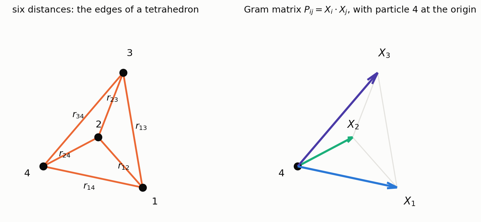
On the left are the six distances as the edges of a tetrahedron. On the right is the same configuration seen from particle 4: three arrows $X_1, X_2, X_3$, and the Gram matrix just records their lengths and the angles between them. Six distances in, six independent entries of a symmetric $3\times 3$ matrix out.

Here is the code I used throughout:

import itertools
import numpy as np
import sympy as sp

rng = np.random.default_rng(1)

# Six interparticle distances of four particles, always in this order
PAIRS = [(1, 2), (1, 3), (1, 4), (2, 3), (2, 4), (3, 4)]
IDX = {p: k for k, p in enumerate(PAIRS)}


def sq(s, i, j):
    """Squared distance between particles i and j from the vector s = r**2."""
    return s[IDX[(min(i, j), max(i, j))]]


def gram(s):
    """Gram matrix of the three vectors X_i = x_i - x_4 (particle 4 at the origin).
    It is LINEAR in the squared distances s."""
    return np.array([[(sq(s, i, 4) + sq(s, j, 4) - (sq(s, i, j) if i != j else 0)) / 2
                      for j in (1, 2, 3)] for i in (1, 2, 3)])


def dists2(x):
    """Squared distances of four points x (4 x dim array)."""
    return np.array([np.sum((x[i - 1] - x[j - 1]) ** 2) for i, j in PAIRS])


def realizable(r, tol=1e-12):
    """Six distances describe four points in 3D  <=>  the Gram matrix is PSD."""
    return np.linalg.eigvalsh(gram(np.asarray(r) ** 2)).min() > -tol


# Schoenberg's theorem, checked on random tetrahedra
for _ in range(1000):
    x = rng.normal(size=(4, 3))
    X = x[:3] - x[3]
    assert np.allclose(gram(dists2(x)), X @ X.T)
print("Gram matrix = X X^T for 1000 random tetrahedra: OK")

Gram matrix = X X^T for 1000 random tetrahedra: OK

This reformulation turns out to be the foundation of everything that follows. In squared distances, the set of possible tetrahedra is a linear copy of the cone of $3\times3$ positive semidefinite matrices. That is a very well understood object, which means we can actually prove things about it (hopefully…)

My first move: stop tripping up over the word “exist”

The thing that caused the biggest issue for me when reading the history of this problem is that everyone was right about something. Jug’s non-existence and Frolov’s existence claims can both be “true” if they are about different properties. So before trying to prove anything, I wrote down a ladder of definitions, from strongest to weakest, and decided to attempt to settle each rung separately.

Rung	What we ask for	Pekeris’ 3-body coordinates?
L1	distances linear in six coordinates ranging over $[0,\infty)^6$	yes
L2	a map that is smooth right up to the boundary (corners to corners, edges to edges)	yes
L3	independent coordinates, smooth inside, every configuration reached	yes
L4	distances are rational functions (e.g. polynomials) of independent coordinates	yes

Pekeris’ coordinates sit on every rung at once so which rungs survive for four bodies?

I also wanted every step to leave behind a runnable check, because this is exactly the kind of problem where a confident-sounding argument can be quietly wrong (Frolov 2006 is proof of that). Every claim below has an assert behind it in checks.py.

Rung 1: linear coordinates are impossible

This one is the easiest, and it is due to Kreuter’s thesis. The picture says it all.

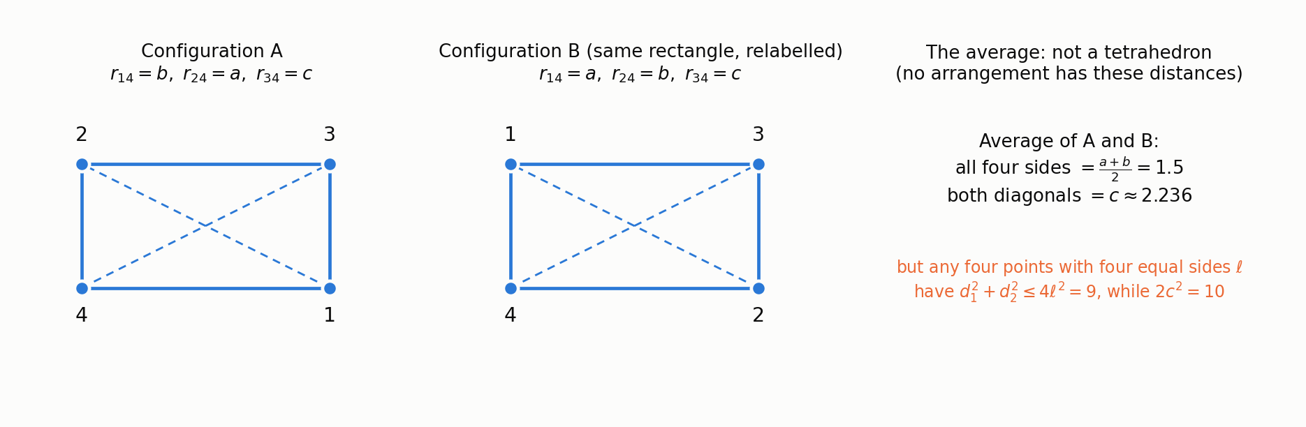
Take four particles at the corners of a flat $a \times b$ rectangle with diagonal $c$. That is a perfectly good (if flat) configuration. Now relabel the corners, so that particles 1 and 2 swap places. That is also a perfectly good configuration with the same shape. Average the two lists of distances and you get four “sides” of length $\tfrac{a+b}{2}$ and two “diagonals” of length $c$.

No arrangement of four points has those distances. For any four points joined in a cycle by four equal sides of length $\ell$, the two diagonals satisfy $d_1^2 + d_2^2 \le 4\ell^2$, with equality only for a flat rhombus. Here $4\ell^2 = 9$ but $2c^2 = 10$.

Why does this kill linear coordinates? If the distances were linear functions of coordinates ranging over a box, then the set of allowed distance vectors would be the image of a box under a linear map, which is a convex shape: the average of any two allowed points would be allowed. We have just found two allowed points whose average is not allowed.

a, b = 1.0, 2.0
c = np.hypot(a, b)                       # diagonal of an a x b rectangle
RA = np.array([c, b, a, a, b, c])        # rectangle, particle 4 at a corner
RB = np.array([c, a, b, b, a, c])        # the same rectangle, relabelled
mid = (RA + RB) / 2

print("rectangle A realizable:", realizable(RA))
print("rectangle B realizable:", realizable(RB))
print("their average realizable:", realizable(mid))
print("smallest Gram eigenvalue of the average:", np.linalg.eigvalsh(gram(mid ** 2)).min())

rectangle A realizable: True
rectangle B realizable: True
their average realizable: False
smallest Gram eigenvalue of the average: -0.34057287393430585

That settles Frolov’s 2006 coordinates; they are linear, so their six constraints can only ever describe a convex region, and the true domain isn’t one.

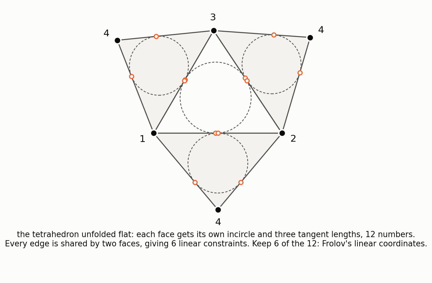
For the record, I think this is what his construction looks like. Unfold the tetrahedron into its four faces, draw each face’s incircle, and you get three tangent lengths per face, twelve numbers in all. Each edge is shared by two faces, so the twelve satisfy six linear “the two halves of this edge add up to the same length” constraints. Keep six of them and you have six perimetric-looking coordinates. The trouble is that every face being a good triangle does not make the four faces fold up into a real tetrahedron.

Why three bodies get away with it

I like having a one-line reason for things, and here it is. For a single triangle, the “is this a real triangle?” test is Heron’s formula for the area, and Heron’s expression factorises into four linear pieces:

\[16A^2 = (r_{12}+r_{13}+r_{23})(-r_{12}+r_{13}+r_{23})(r_{12}-r_{13}+r_{23})(r_{12}+r_{13}-r_{23}).\]

Three of those linear factors are exactly the perimetric coordinates. The boundary of the triangle domain is a set of flat walls, and flat walls can be straightened into the walls of a box by a linear map.

For the tetrahedron, the “is this a real tetrahedron?” test is the Cayley–Menger determinant, and it does not factorise at all. It is a single irreducible polynomial of degree six in the distances, so its boundary is curved.

r12, r13, r14, r23, r24, r34 = R = sp.symbols('r12 r13 r14 r23 r24 r34', positive=True)
P = sp.Matrix([[r14**2, (r14**2 + r24**2 - r12**2) / 2, (r14**2 + r34**2 - r13**2) / 2],
               [(r14**2 + r24**2 - r12**2) / 2, r24**2, (r24**2 + r34**2 - r23**2) / 2],
               [(r14**2 + r34**2 - r13**2) / 2, (r24**2 + r34**2 - r23**2) / 2, r34**2]])

triangle = sp.factor(P[:2, :2].det())    # one face of the tetrahedron (a triangle)
print("triangle (Heron):", triangle)

tet = sp.factor_list(sp.expand(P.det()))  # the whole tetrahedron (Cayley-Menger)
print("tetrahedron: number of factors =", len(tet[1]),
      "| degree =", sp.Poly(tet[1][0][0], *R).total_degree())

triangle (Heron): -(r12 - r14 - r24)*(r12 - r14 + r24)*(r12 + r14 - r24)*(r12 + r14 + r24)/4
tetrahedron: number of factors = 1 | degree = 6

That is the whole story of perimetric coordinates in two lines, four linear factors for the triangle, one irreducible sextic for the tetrahedron.

Rung 2: smooth-to-the-boundary coordinates are impossible

The next question I asked was: fine, the distances can’t be linear, but could there be a cleverer, curved map that still behaves like Pekeris’ at the edges? Pekeris’ map sends corners of the box to corners of the domain and flat faces to flat faces, and it is smooth with a non-degenerate Jacobian everywhere, including on the boundary.

Here is the obstruction, and I find it quite visual. Think about what the edge of the domain looks like near a very special configuration: all four particles in a straight line. I find these proofs become simpler to follow when we assume a bizaare, but physical orientation…

• Near any point of a box, the edge looks like a corner made of flat walls: a half-space, a right-angled wedge, or a three-walled corner
• Near four collinear particles, the edge of the tetrahedron domain looks like the inside of an ice-cream cone: a round cone, ${ac \ge b^2,\ a,c \ge 0}$, crossed with some flat directions

A smooth map with an invertible Jacobian sends the “local shape” of the edge at one point to the local shape at the image point by a linear map, and a linear map can never turn flat walls into a round cone. So no such map exists, and the obstruction is purely local and it happens near every single collinear configuration.

I wanted to visualise that cone rather than take it on trust, so I generated real configurations. Start from four particles on a line, jiggle them a little in random directions, and compute their Gram matrix. Most of the Gram matrix just measures how long the line is, which is boring. What is left over, the part that says how far the particles stick out sideways from the line, is a $2\times 2$ symmetric matrix $\begin{pmatrix} a & b \ b & c\end{pmatrix}$ (a Schur complement, if you want the proper name). It is positive semidefinite exactly when the configuration is genuine, and that condition, $ac \ge b^2$ with $a, c\ge 0$, is a round cone in disguise: with $x = (a-c)/2$, $y = b$, $z = (a+c)/2$ it reads $z \ge \sqrt{x^2+y^2}$.

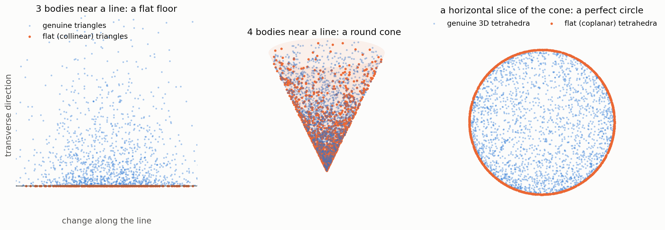
Every dot is a real configuration of particles. On the left, the same experiment for three bodies near a line: the flat (collinear) triangles all land on a straight floor, a flat wall just like the edge of Pekeris’ octant. In the middle, four bodies: the flat (coplanar) tetrahedra in orange coat the surface of an ice-cream cone and the genuine 3D ones fill its inside. On the right I sliced the cone horizontally and the flat tetrahedra land on a perfect circle, to nine decimal places, and they hit every part of it. A box corner sliced the same way would give a polygon with straight sides. You cannot bend a polygon into a circle with a smooth invertible map.

def transverse_block(G, vhat):
    """2x2 Schur complement of the Gram matrix across the collinear direction vhat.
    PSD exactly when G is, singular exactly when the configuration is flat."""
    Q = np.linalg.qr(np.column_stack([vhat, np.eye(3)]))[0]
    Gq = Q.T @ G @ Q
    return Gq[1:, 1:] - np.outer(Gq[1:, 0], Gq[0, 1:]) / Gq[0, 0]


def cone_slice(x, vhat):
    """PSD 2x2 matrices [[a, b], [b, c]] are the round cone z >= sqrt(x^2 + y^2) with
    (x, y, z) = ((a - c)/2, b, (a + c)/2). Return the point on the slice z = 1."""
    C = transverse_block(gram(dists2(x)), vhat)
    a, b, c = C[0, 0], C[0, 1], C[1, 1]
    return np.array([(a - c) / 2, b]) / ((a + c) / 2)


eps = 0.02
vhat = (x0[:3] - x0[3])[:, 0] / np.linalg.norm((x0[:3] - x0[3])[:, 0])
genuine = np.array([cone_slice(x0 + rng.normal(size=(4, 3)) * eps, vhat) for _ in range(2000)])
flat = []
for _ in range(2000):
    phi = rng.uniform(0, np.pi)                       # a random plane through the line
    d = np.outer(rng.normal(size=4) * eps, [0, np.cos(phi), np.sin(phi)])
    d[:, 0] += rng.normal(size=4) * eps
    flat.append(cone_slice(x0 + d, vhat))
flat = np.array(flat)
radius_flat = np.linalg.norm(flat, axis=1)
angles_hit = np.unique((np.degrees(np.arctan2(flat[:, 1], flat[:, 0])) // 10).astype(int))
print("genuine tetrahedra strictly inside the circle:", bool(np.linalg.norm(genuine, axis=1).max() < 1))
print("flat tetrahedra: largest |radius - 1| =", f"{np.abs(radius_flat - 1).max():.1e}")
print("10-degree sectors of the circle hit by flat tetrahedra:", len(angles_hit), "of 36")

genuine tetrahedra strictly inside the circle: True
flat tetrahedra: largest |radius - 1| = 1.4e-09
10-degree sectors of the circle hit by flat tetrahedra: 36 of 36

The code that draws the figures, including this one, is make_diagrams.py in the code folder.

To check this numerically I nudged four collinear particles into slightly different flat (coplanar) arrangements and computed the outward normal of the domain’s boundary at each. Near a flat-walled corner you would only ever see a handful of distinct normals, one per wall but near the ice-cream cone you see a continuum.

detP = sp.lambdify(R, P.det())
grad = sp.lambdify(R, [sp.diff(P.det(), v) for v in R])

x0 = np.array([[0., 0, 0], [1, 0, 0], [2.5, 0, 0], [4, 0, 0]])   # four collinear particles
normals = []
for th in np.linspace(0, np.pi, 40, endpoint=False):
    x = x0.copy()
    x[1, 1], x[2, 1] = 1e-4 * np.cos(th), 1e-4 * np.sin(th)        # nudge into a plane
    r = np.sqrt(dists2(x))
    g = np.array(grad(*r))
    normals.append(g / np.linalg.norm(g))
normals = np.array(normals)
gap = min(min(np.linalg.norm(u - v), np.linalg.norm(u + v))
          for u, v in itertools.combinations(normals, 2))
print("40 boundary normals within 1e-4 of a collinear configuration")
print("smallest angle-gap between any two of them:", round(gap, 4), "(all distinct)")

40 boundary normals within 1e-4 of a collinear configuration
smallest angle-gap between any two of them: 0.0445 (all distinct)

Another observation that surprised me is that for the triangle a degenerate (flat) triangle is a corner of the domain. For the tetrahedron a degenerate face (three particles in a line, the fourth off it) is not a corner. It is a perfectly smooth point of the boundary, the tetrahedron’s domain is rounder than you (I certainly) would naively expect.

Rung 3: independent coordinates do exist

At this point it would be tempting to declare “they don’t exist” and go to bed (which, by the way, I did do several times), but that is what the literature also did, because the weaker version of the question has a positive answer.

Remember that in squared distances the domain is a copy of the positive semidefinite cone. Every positive semidefinite matrix has a Cholesky factorisation $P = LL^T$ with $L$ lower-triangular,

\[L = \begin{pmatrix} l_{11} & 0 & 0 \\ l_{21} & l_{22} & 0 \\ l_{31} & l_{32} & l_{33} \end{pmatrix},\]

where the diagonal entries are $\ge 0$ and the off-diagonal entries can be any real number. That is already six independent coordinates on a product domain $[0,\infty)^3\times\mathbb{R}^3$, the squared distances are quadratic polynomials of them, and every configuration is reached exactly once (for non-flat ones). This is essentially Carter’s 1968 “normal” coordinates.

If you insist on six coordinates that all live on $[0,\infty)$, as Pekeris’ do, there is a cute little fix. Squaring a complex number $z = q_a + i q_b$ maps the quarter-plane $q_a, q_b \ge 0$ onto the upper half-plane, one-to-one. So each pair (real off-diagonal entry, non-negative diagonal entry) can be produced as (real part, imaginary part) of $z^2$:

\[l_{21} + i\,l_{11} = (q_1 + i q_2)^2,\qquad l_{31} + i\,l_{22} = (q_3 + i q_4)^2,\qquad l_{32} + i\,l_{33} = (q_5 + i q_6)^2 .\]

The squared distances become degree-4 polynomials in six coordinates $q\in[0,\infty)^6$, every tetrahedron is reached, and the map is one-to-one on the interior.

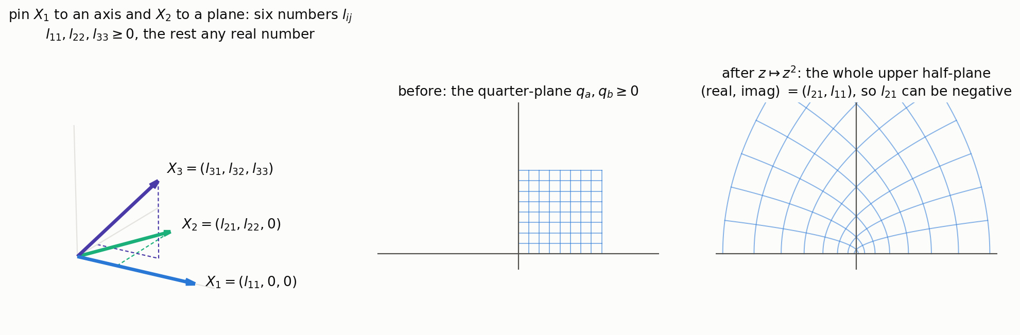
On the left is what the Cholesky coordinates mean geometrically: rotate the whole configuration so that $X_1$ points along the $x$-axis and $X_2$ lies in the $xy$-plane. What is left are six honest numbers, the components that the rotation could not kill. On the right is the $z^2$ trick: the square grid of the quarter-plane gets opened out like a fan into the whole upper half-plane, so two coordinates that live on $[0,\infty)$ produce one coordinate that is $\ge 0$ and one that can take any sign.

def L_of_q(q):
    """Lower-triangular Cholesky factor built from six coordinates q >= 0.
    Each (off-diagonal, diagonal) pair is (Re, Im) of z^2 with z = q_a + i q_b."""
    z = [complex(q[2 * k], q[2 * k + 1]) ** 2 for k in range(3)]
    L = np.zeros((3, 3))
    L[0, 0], L[1, 0] = z[0].imag, z[0].real
    L[1, 1], L[2, 0] = z[1].imag, z[1].real
    L[2, 2], L[2, 1] = z[2].imag, z[2].real
    return L


def s_of_q(q):
    """Squared distances (degree-4 polynomials in q) from the Gram matrix L L^T."""
    G = L_of_q(q) @ L_of_q(q).T
    s = np.empty(6)
    s[IDX[(1, 4)]], s[IDX[(2, 4)]], s[IDX[(3, 4)]] = np.diag(G)
    for i, j in ((1, 2), (1, 3), (2, 3)):
        s[IDX[(i, j)]] = G[i - 1, i - 1] + G[j - 1, j - 1] - 2 * G[i - 1, j - 1]
    return s


def q_of_s(s):
    """Inverse map: Cholesky factor, then the principal square root of each pair."""
    L = np.linalg.cholesky(gram(s))
    w = [np.sqrt(complex(o, d)) for d, o in ((L[0, 0], L[1, 0]), (L[1, 1], L[2, 0]), (L[2, 2], L[2, 1]))]
    return np.array([c for x in w for c in (x.real, x.imag)])


worst = 0
for _ in range(1000):
    q = rng.uniform(0.2, 3.0, size=6)
    s = s_of_q(q)
    assert realizable(np.sqrt(s))
    worst = max(worst, np.max(np.abs(q_of_s(s) / q - 1)))
print("1000 random q in the open orthant -> valid tetrahedra -> back to q")
print("worst relative round-trip error:", f"{worst:.1e}")

1000 random q in the open orthant -> valid tetrahedra -> back to q
worst relative round-trip error: 4.4e-13

Even the integration measure comes out polynomial, $d\tau \propto 8\,l_{11}^2\,l_{22}\prod_k 4(q_{2k-1}^2+q_{2k}^2)\,dq$.

So independent four-body coordinates do exist, but look carefully at what we get. The squared distances are polynomials, and the distances themselves are $r_{ij} = \sqrt{\text{polynomial}}$, which, for a Coulomb problem, is fatal as the potential is $1/r_{ij}$ and the good basis functions contain $e^{-\alpha r_{ij}}$. THis results in square roots everywhere which brings us to the next question.

Rung 4: can the distances themselves be rational?

I think this is the version that matters for computation, and I think it is the version everybody actually had in mind. Can we find six independent coordinates, ranging over a box, such that the six distances are rational functions (ratios of polynomials, in particular polynomials) of them?

The answer is no, and the reason took me down a rabbit hole.

Step 1: turning it into a question about the boundary

Suppose such coordinates existed. The box has flat faces, and each face of the box must be sent onto the boundary of the domain: the flat, coplanar configurations. (If a face point landed inside the domain, two different interior points would end up with the same image, which a classic topological result called invariance of domain forbids.)

A flat face of a box is about the simplest shape there is, a chunk of ordinary flat space. So if a rational map sent it onto the coplanar boundary, we would have a rational parametrisation of the set of flat four-particle configurations, written in the distances. The algebraic geometers call a shape with that property unirational (your word of the day).

So the question now reduces to:

can the coplanar configurations, written in terms of the six distances, be parametrised by rational functions?

An analogy: the circle and the doughnut

Here is the intuition I found most helpful, a circle can be parametrised by rational functions:

\[t \;\mapsto\; \left(\frac{1-t^2}{1+t^2},\ \frac{2t}{1+t^2}\right).\]

The curve $y^2 = x^3 - x$ cannot. Over the complex numbers, this curve is a doughnut (a torus), and a doughnut carries a special everywhere-nonzero “holomorphic form” that any rational parametrisation would be forced to destroy. Shapes with these forms are allergic to rational parametrisations.

Keep that curve $y^2 = x^3 - x$ in mind, because it is going to come back. Later on I will show it turning up in real data.

Step 2: the null-coordinate trick

The distances live on a complicated shape, so I wanted coordinates in which they become simple. For a flat configuration, put each particle in the complex plane and use the “null coordinates”

\[z = x + iy,\qquad w = x - iy .\]

Then a squared distance factorises:

\[|\mathbf{x}_a - \mathbf{x}_b|^2 = (z_a - z_b)(w_a - w_b).\]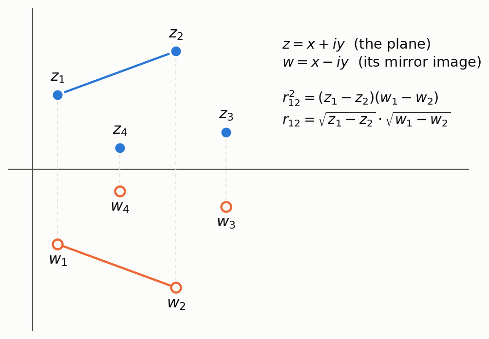

For real particles, $w$ is just the mirror image of $z$ and the trick is to stop treating them as linked and let them be two independent sets of numbers. Then every squared distance is a product of a pure-$z$ piece and a pure-$w$ piece, and the problem splits in two.

So $r_{ab} = \sqrt{z_a - z_b}\cdot\sqrt{w_a - w_b}$, and the six distances split into “a $z$-part” times “a $w$-part”. Define $\alpha_{ij} = \sqrt{z_j - z_i}$. Because $(z_2 - z_1) + (z_3 - z_2) = (z_3 - z_1)$, the six numbers $\alpha_{ij}$ satisfy three equations that look like Pythagoras’ theorem:

\[\alpha_{12}^2+\alpha_{23}^2=\alpha_{13}^2,\qquad \alpha_{12}^2+\alpha_{24}^2=\alpha_{14}^2,\qquad \alpha_{13}^2+\alpha_{34}^2=\alpha_{14}^2 .\]

These three equations define a surface $X$. The coplanar boundary we care about is, up to some symmetries (sign changes and swapping $z\leftrightarrow w$), just two copies of $X$ glued together via $r_{ij} = \alpha_{ij}\beta_{ij}$.

# X: three diagonal quadrics in P^5  (alpha_ij^2 = z_j - z_i, written without z)
QX = np.array([[1, -1, 0, 1, 0, 0],    # a12^2 + a23^2 - a13^2 = 0
               [1, 0, -1, 0, 1, 0],    # a12^2 + a24^2 - a14^2 = 0
               [0, 1, -1, 0, 0, 1]])   # a13^2 + a34^2 - a14^2 = 0


def point_on_X(z):
    """A point of X from four complex numbers z_1..z_4 (null coordinates)."""
    return np.sqrt(np.array([z[j - 1] - z[i - 1] for i, j in PAIRS], dtype=complex))


for _ in range(1000):
    al = point_on_X(rng.normal(size=4) + 1j * rng.normal(size=4))
    be = point_on_X(rng.normal(size=4) + 1j * rng.normal(size=4))
    assert np.allclose(QX @ al ** 2, 0) and np.allclose(QX @ be ** 2, 0)
    r = al * be                                        # r_ij = alpha_ij * beta_ij
    assert abs(np.linalg.det(gram(r ** 2))) < 1e-10 * np.abs(r).max() ** 6
print("1000 random pairs (alpha, beta) on X x X give r with Cayley-Menger = 0: OK")

1000 random pairs (alpha, beta) on X x X give r with Cayley-Menger = 0: OK

Step 3: $X$ is a K3 surface

Now the question is what kind of surface $X$ is. Three quadratic equations in six homogeneous variables cut out what is called a K3 surface and in order to tackle this nect problem I had to learn what they are. K3 surfaces are the two-dimensional cousins of the doughnut, carrying exactly one everywhere-nonzero holomorphic 2-form, and that form makes them allergic to rational parametrisation, just like the torus.

There is a small subtlety though, our $X$ is not perfectly smooth. It has a few pinched points, and I needed to check that they are the harmless kind (simple “double points” that do not spoil the K3 structure). The code finds them by checking where the equations stop being independent

E = sp.Matrix([[(m == j) - (m == i) for m in (1, 2, 3, 4)] for i, j in PAIRS])
ones = sp.Matrix([1, 1, 1, 1])
supports = {tuple(range(6))} | {tuple(k for k in range(6) if k != m) for m in range(6)}
for f, g in itertools.combinations(range(6), 2):
    z = [v for v in sp.Matrix.vstack(E[f, :], E[g, :]).nullspace()
         if sp.Matrix.hstack(v, ones).rank() == 2][0]
    vals = E * z
    supports.add(tuple(k for k in range(6) if vals[k] != 0))
singular = [S for S in supports if sp.Matrix(QX)[:, list(S)].rank() < 3]
print("singular supports:", singular)
print("number of singular points:", sum(2 ** len(S) // 2 for S in singular))

singular supports: [(0, 1, 2), (1, 3, 5), (2, 4, 5), (0, 3, 4)]
number of singular points: 16

Sixteen double points result. That number is a fingerprint in its own right as a K3 surface with exactly sixteen such points is a Kummer surface, the kind you get by taking a product of two doughnuts and folding it in half (yummy).

Step 4: the contradiction

Put it together:

• the coplanar boundary is (birationally) $X\times X$ folded by a finite group of symmetries,
• each copy of $X$ carries a holomorphic 2-form, so $X\times X$ carries a holomorphic 4-form,
• the symmetries are all sign flips, and the 4-form survives the folding (a sign flip on each copy multiplies the form by $(\pm1)^2 = +1$),
• so the coplanar boundary carries a holomorphic 4-form, which no rational parametrisation can produce.

Therefore no rational perimetric coordinates exist! In the paper version which I may upload at some point this is Theorem 6.1, and it applies to any box, simplex, polyhedron or ball you might choose as the coordinate domain. It even applies piecewise.

A sanity check from number theory

I did not want to trust the “it’s a K3 surface” step on theory alone, so I asked for an independent fingerprint. If you count the points of $X$ over a finite field $\mathbb{F}_p$ (arithmetic modulo a prime $p$), a surface that could be rationally parametrised always gives a count of 1 modulo $p$ (a theorem of Esnault). A K3 surface typically does not.

def legendre_symbol(p):
    chi = -np.ones(p, int)
    chi[0] = 0
    chi[(np.arange(1, p) ** 2) % p] = 1
    return chi


def count_points(p, n=4):
    """Projective points of X over F_p: fix z_1 = 0, run over the other z's, and weight
    each choice by the number of square roots alpha_ij = sqrt(z_j - z_i) it allows."""
    chi = legendre_symbol(p)
    z = [np.zeros((p,) * (n - 1), int)] + list(np.indices((p,) * (n - 1)))
    prod = np.ones((p,) * (n - 1), int)
    for i, j in itertools.combinations(range(n), 2):
        prod *= 1 + chi[(z[j] - z[i]) % p]          # number of square roots
    return (int(prod.sum()) - 1) // (p - 1)         # projective points


print(" p   #X(F_p)   mod p   1 + 2(a^2 - b^2) mod p")
for p in (7, 11, 13, 17, 19, 29, 37, 41):
    n = count_points(p)
    if p % 4 == 3:
        print(f"{p:3d} {n:8d} {n % p:7d}   (p = 3 mod 4: #X = (p+1)^2 = {(p + 1) ** 2})")
    else:
        a_, b_ = next((a_, b_) for a_ in range(1, p, 2) for b_ in range(0, p, 2) if a_ * a_ + b_ * b_ == p)
        print(f"{p:3d} {n:8d} {n % p:7d}   {(1 + 2 * (a_ * a_ - b_ * b_)) % p:5d}")
print("control (three bodies, a conic):", [bool(count_points(p, 3) == p + 1) for p in (13, 17, 29)])

 p   #X(F_p)   mod p   1 + 2(a^2 - b^2) mod p
  7       64       1   (p = 3 mod 4: #X = (p+1)^2 = 64)
 11      144       1   (p = 3 mod 4: #X = (p+1)^2 = 144)
 13      232      11      11
 17      328       5       5
 19      400       1   (p = 3 mod 4: #X = (p+1)^2 = 400)
 29     1000      14      14
 37     1448       5       5
 41     1864      19      19
control (three bodies, a conic): [True, True, True]

The counts are not 1 mod $p$ whenever $p \equiv 1 \pmod 4$, so $X$ cannot be rationally parametrised, independently of the holomorphic-form argument. I think this pattern is quite beautiful, writing $p = a^2 + b^2$, the count is $1 + 2(a^2-b^2)$ modulo $p$, and $2(a^2 - b^2)$ is exactly the $p$-th coefficient of a famous modular form, $\eta(4\tau)^6$. That form is attached to the doughnut $y^2 = x^3 - x$ from the analogy above.

Once I had the data I could not resist pushing further, and it turned out the relationship is not just a congruence modulo $p$, it is an exact formula. Count the points of the doughnut $E: y^2 = x^3 - x$ over $\mathbb{F}_p$ and write the answer as $p + 1 - a_p$. Then for every prime I tried,

\[|X(\mathbb{F}_p)| = (p+1)^2 + a_p^2 .\]

The $(p+1)^2$ is what a rational shape (two copies of a line) would give, and the $a_p^2$ is the doughnut’s signal, squared because $X$ is built from two copies of it. When $p \equiv 3 \pmod 4$ the doughnut happens to have $a_p = 0$, which is why those rows of the table looked so innocent.

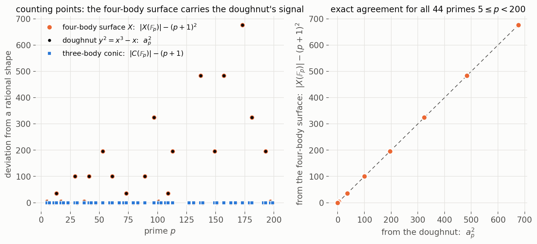
The left panel shows the deviation from “rational behaviour” for each prime: the four-body surface (orange) sits exactly on the doughnut’s numbers (black), while the three-body conic (blue) never moves off zero. The right panel plots one against the other, and all 44 primes between 5 and 200 land on the diagonal. This is the doughnut from the analogy section, measured directly.

def a_p(p):
    """#E(F_p) = p + 1 - a_p for the curve E: y^2 = x^3 - x."""
    x = np.arange(p)
    return -int(legendre_symbol(p)[(x ** 3 - x) % p].sum())


primes = list(sp.primerange(5, 200))
assert all(count_points(p) == (p + 1) ** 2 + a_p(p) ** 2 for p in primes)
assert all(count_points(p, 3) == p + 1 for p in primes)
print(f"|X(F_p)| = (p+1)^2 + a_p^2 for all {len(primes)} primes 5 <= p < 200")
print("first few a_p:", {p: a_p(p) for p in primes[:8]})

|X(F_p)| = (p+1)^2 + a_p^2 for all 44 primes 5 <= p < 200
first few a_p: {5: -2, 7: 0, 11: 0, 13: 6, 17: 2, 19: 0, 23: 0, 29: -10}

The three-body control is a conic (a circle in disguise) and gives exactly $p+1$ points, i.e. $1$ mod $p$, as a rationally parametrisable shape must. That is the difference between three and four bodies in one table.

But could we still be fast?

Having killed rational distances, I still had a nagging question. Pekeris did not need linear distances for their own sake, he needed his matrix to be sparse: a fixed number of nonzero entries per row, no matter how big the basis. Maybe there is another route to sparsity that does not need rational distances?

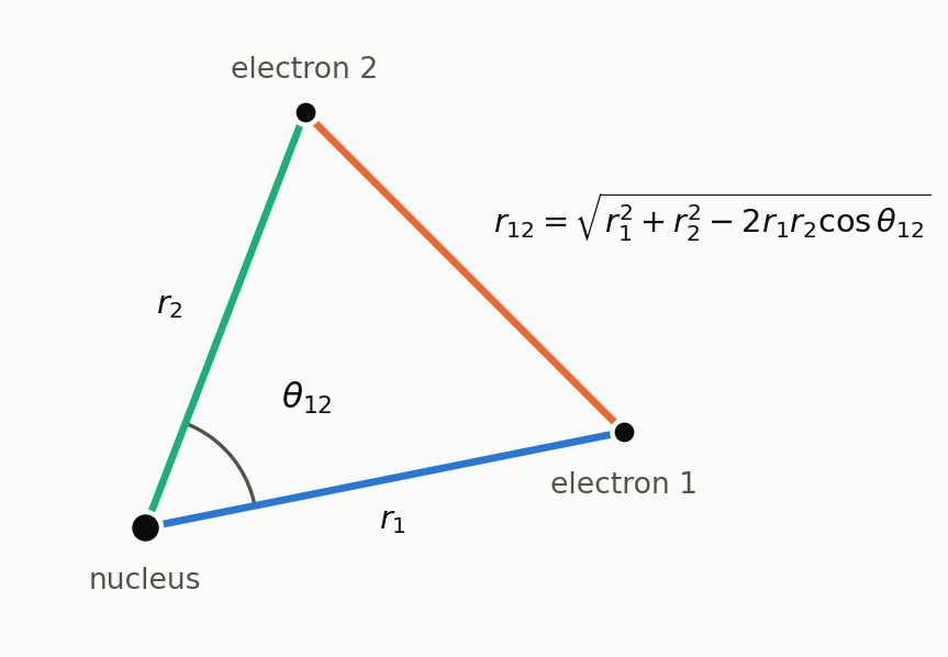
The test case is helium, where the standard coordinates are the two electron–nucleus distances $r_1, r_2$ and the angle $\theta_{12}$ between them. In these coordinates the electron–electron distance $r_{12}$ is a square root, exactly the situation four bodies leave us in.

My idea is as follows. Use coordinates where only the squared distances are polynomial (rung 3 says these exist), and handle the square roots by splitting the wavefunction into an “even” and an “odd” part. For helium in $(r_1, r_2, \cos\theta_{12})$ coordinates that means writing

\[\Psi = e^{-(x_1+x_2)/2}\left[f_0(x_1,x_2,c) + r_{12}\,f_1(x_1,x_2,c)\right],\]

where $f_0$ and $f_1$ are expanded in Laguerre × Laguerre × Legendre polynomials. The trick is that differentiating $r_{12}$ or dividing by it never leaves this “even plus $r_{12}$ times even” family, because $\partial r_{12} = \partial(r_{12}^2)/(2r_{12})$ and $1/r_{12} = r_{12}/r_{12}^2$. So the Hamiltonian maps the family into itself with polynomial coefficients, and every term acts on the Laguerre and Legendre basis with a short stencil. That is exactly the Pekeris structure.

I built it (he_graded.py), and checked the operator symbolically against the real Schrödinger equation at random points, so I knew the algebra was right. The sparsity was perfect: at most 188 nonzeros per row, however large the basis. Then I computed the energy.

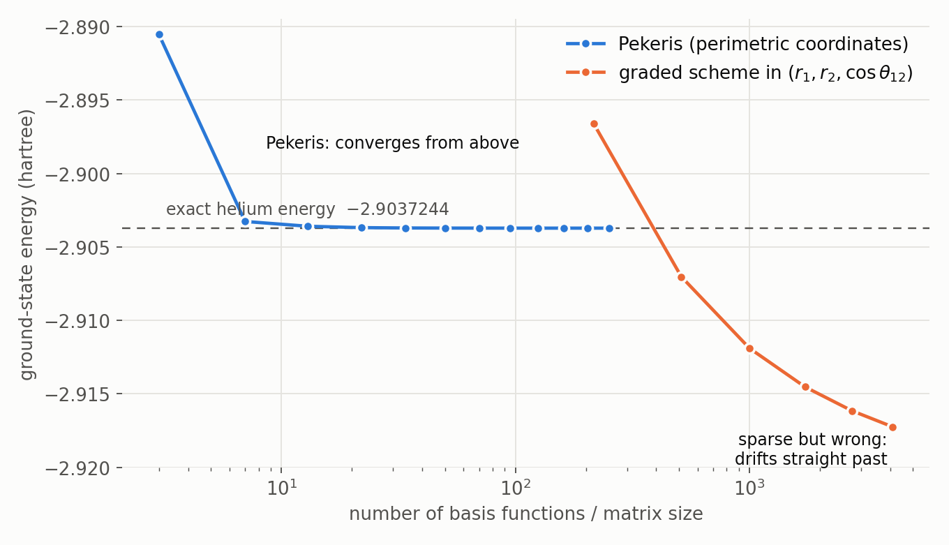
The Pekeris curve (blue, the data from my earlier post) converges from above, as a variational method should. The graded scheme (orange) sails straight through the exact energy and keeps falling. It is sparse, it is algebraically correct, and it is wrong.

It took me a while to see why, and the answer is genuinely lovely. Look at how the sparse matrix is assembled:

A = sps.bmat([[r(A00), lam * r(Mx)], [lam * r(Mx), r(A11)]], format='csr')
B = sps.bmat([[r(B00), None], [None, r(B11)]], format='csr')

The electron–electron repulsion strength lam only appears in the off-diagonal blocks. Flip the sign of the odd block (multiply by $-1$) and lam becomes -lam, but the spectrum does not change. In words: the scheme computes exactly the same energies for electrons that repel and electrons that attract. Real helium and “helium with attractive electrons” obviously have different energies, so the scheme cannot be converging to either of them.

import scipy.linalg as sla
from he_graded import operators

for lam in (+1.0, -1.0):
    A, B, _ = operators(6, 3, Z=2.0, kappa=1.0, lam_ee=lam)
    w = sla.eigvals(A.toarray(), B.toarray()) * 4
    w = np.sort(w[np.isfinite(w) & (np.abs(w.imag) < 1e-9)].real)
    print(f"e-e coupling {lam:+.0f}: lowest real eigenvalues", np.round(w[:4], 6))

e-e coupling +1: lowest real eigenvalues [-4.862116 -2.971481 -2.896608 -2.780091]
e-e coupling -1: lowest real eigenvalues [-4.862116 -2.971481 -2.896608 -2.780091]

Identical, to every digit.

The deeper reason is a piece of Galois theory. Every quantity the sparse scheme computes is a rational function of the coordinates, and replacing $r_{12}$ by $-r_{12}$ leaves all of those untouched. The only thing that changes sign under that swap is the Coulomb term $1/r_{12}$. The physical inner product, $\int \psi\,H\,\phi\,d\tau$, does notice the swap, but only through integrals of $r_{12}$ times polynomials, which are not polynomial, and those are precisely the integrals that make the matrix dense again.

Pekeris escapes because in perimetric coordinates $r_{12}$ is linear, so there is no square root to swap. For four bodies, this means:

• a Pekeris-type sparse method needs every distance to be a rational function of the coordinates, otherwise the Galois swap makes it blind to the sign of that pair’s Coulomb interaction,
• and rung 4 says that is impossible for four bodies.

So, within this framework, there is no Pekeris-type method for four-body Coulomb systems. Two quite different pieces of mathematics, algebraic geometry and Galois theory, end up blocking us at the same door.

Side quest: how simple can the squared distances be?

Rung 3 gave squared distances that are degree-4 polynomials. For three bodies, Pekeris’ squared distances are degree 2, $s_{ij} = (u_i + u_j)^2$. So I could not resist asking: what is the lowest possible degree for four bodies?

I will keep this short because it is the most technical part, but the summary is:

• Degree 2 is impossible (for coordinates that scale with the system, like Pekeris’). The proof chains a degree count, a local analysis of where collinear configurations can sit, and some algebraic topology that reduces everything to a finite check: which collections of triangles inside a 6-vertex simplex can “wrap around” the projective plane of possible collinear directions? The answer is exactly 12, and they are all copies of the hemi-icosahedron (an icosahedron with opposite faces identified, so many words of the day today).
• Degree 3 is open. I ruled out every family I could think of, including anything built as a sum of three weighted rank-one terms, and anything with the icosahedral symmetry the topology hints at. My conjecture is that 4 is the minimum.

The enumeration that finds the hemi-icosahedra is short enough to show:

def nullspace_mod2(M):
    M = M.copy() % 2
    rows, cols = M.shape
    piv, r = [], 0
    for c in range(cols):
        p = next((i for i in range(r, rows) if M[i, c]), None)
        if p is None:
            continue
        M[[r, p]] = M[[p, r]]
        for i in range(rows):
            if i != r and M[i, c]:
                M[i] ^= M[r]
        piv.append(c)
        r += 1
    out = []
    for f in (c for c in range(cols) if c not in piv):
        x = np.zeros(cols, np.int64)
        x[f] = 1
        for i, pc in enumerate(piv):
            x[pc] = M[i, f]
        out.append(x % 2)
    return out


EDGES = list(itertools.combinations(range(6), 2))
EI = {e: i for i, e in enumerate(EDGES)}
TRIS = list(itertools.combinations(range(6), 3))
TE = [[EI[(a, b)], EI[(b, c)], EI[(a, c)]] for a, b, c in TRIS]

boundary = np.zeros((15, 20), np.int64)
for t in range(20):
    for e in TE[t]:
        boundary[e, t] = 1
cycle_basis = nullspace_mod2(boundary)
print("independent mod-2 2-cycles of the 5-simplex:", len(cycle_basis))

hits = []
for bits in itertools.product([0, 1], repeat=10):
    if not any(bits):
        continue
    z = np.zeros(20, np.int64)
    for bit, v in zip(bits, cycle_basis):
        if bit:
            z ^= v
    tris = [t for t in range(20) if z[t]]
    edges = sorted({e for t in tris for e in TE[t]})
    col = {e: k for k, e in enumerate(edges)}
    D = np.zeros((len(tris), len(edges)), np.int64)
    for row, t in enumerate(tris):
        for e in TE[t]:
            D[row, col[e]] = 1
    for sbits in itertools.product([0, 1], repeat=len(nullspace_mod2(D))):
        sigma = np.zeros(len(edges), np.int64)
        for bit, v in zip(sbits, nullspace_mod2(D)):
            if bit:
                sigma ^= v
        cup = sum(sigma[col[EI[TRIS[t][:2]]]] * sigma[col[EI[TRIS[t][1:]]]] for t in tris) % 2
        if cup == 1:
            hits.append(tuple(TRIS[t] for t in tris))
print("(cycle, sign) pairs carrying the RP^2 class:", len(hits))
print("distinct supporting cycles:", len(set(hits)), "| triangles in each:", {len(h) for h in hits})

independent mod-2 2-cycles of the 5-simplex: 10
(cycle, sign) pairs carrying the RP^2 class: 384
distinct supporting cycles: 12 | triangles in each: {10}

From there, positivity forces the ten triangles not in the hemi-icosahedron to be “flat”, and a final exhaustive check shows that this collapses all six directions into a single plane. That flattens the wrap-around class to zero, which is the contradiction. I enjoyed this part in particular as a question about atoms turned into counting triangles on a hemi-icosahedron.

One honest confession from this stage: my first version of that argument had a gap as I had assumed a certain triple of vectors was always independent, and when I went back to check, the coplanar case slipped through. It is now handled, but it is a good reminder of why we should always insist on leaving a runnable check behind every claim.

So, can we definitively disprove their existence?

For the version of the question that matters, yes, with a precise statement:

There is no system of six independent coordinates, ranging over a box (or any polyhedron or ball), in which the six interparticle distances of a four-body system are rational (in particular, polynomial or linear) functions and every configuration is reached. There is no Pekeris-type sparse method for four-body Coulomb systems in this framework. Independent coordinates do exist, but only with the distances as square roots of polynomials.

Claim	Status
Linear coordinates (Frolov 2006 type)	impossible (elementary)
Coordinates smooth up to the boundary, like Pekeris’	impossible, even locally
Independent coordinates with polynomial squared distances	exist (degree 4)
Independent coordinates with rational distances	impossible
Pekeris-type sparse Coulomb method	impossible in this framework

What would I want before calling it absolutely watertight?

1. An independent check of the K3 step. The identification of the coplanar boundary with $(X\times X)/G$, and the fact that $X$ is a K3 surface, are both standard algebraic geometry and are supported by all the numerics above. They deserve a verification in a dedicated computer algebra system (Macaulay2 or Magma) and an expert pair of eyes.
2. Two loopholes, which are technicalities rather than practical escape routes. One is using more than six coordinates tied together by constraints, which are then no longer “independent”. The other is maps that only reach the boundary at infinity, which does not apply to coordinates that scale like Pekeris’.
3. The primary sources. I could not access the full texts of Rasiel and Karl, White, or Jug, so my account of those papers relies on their abstracts and later citations.

What this means for lithium

The practical consequence is a little sad for our old friend lithium, there is no Pekeris shortcut for four bodies. The methods that actually work for lithium-like systems are the dense ones. These are Hylleraas expansions with clever analytic or recursive three-electron integrals (Fromm and Hill, Remiddi, Harris and successors), and explicitly correlated Gaussians. The Gaussians are interesting in light of rung 3: they live naturally in squared-distance coordinates, and that is exactly the world where four-body coordinates do behave nicely.

What I learned from this project

• Define the question before you answer it. Sixty years of disagreement mostly came from different people having different definitions of the word “exist”
• Climb a ladder of definitions. Settling each rung separately turned one vague question into five sharp ones, some with positive answers
• Look for the hidden object. Here it was a K3 surface sitting inside the set of flat tetrahedra. I did not know what K3 surfaces were but now I do!
• Get an independent fingerprint. The finite-field point count checks the K3 claim by a route that shares nothing with the original argument
• Correct but wrong is a real failure mode. The graded helium scheme was algebraically verified and perfectly sparse, and still converged to the wrong answer. A symmetry check (flip the sign of the repulsion) caught it instantly
• Leave an assertion behind every claim. It caught my own gap in the degree-2 argument

References

• C. L. Pekeris, “Ground State of Two-Electron Atoms”, Phys. Rev. 112, 1649 (1958).
• A. S. Coolidge and H. M. James, Phys. Rev. 51, 855 (1937).
• Y. Rasiel and J. Karl, “Four-particle perimetric coordinates”, Theor. Chim. Acta 5, 179 (1966).
• R. J. White, “Perimetric coordinates for four particles”, Theor. Chim. Acta 6, 450 (1966).
• K. Jug, “Perimeterkoordinaten für Vierteilchensysteme”, Theor. Chim. Acta 7, 167 (1967).
• P. S. C. Wang, “Perimetric Coordinates”, J. Chem. Phys. 47, 2229 (1967).
• B. P. Carter, “Four-Body S-State Coordinates”, J. Chem. Phys. 49, 3683 (1968).
• A. M. Frolov, “Four-body perimetric coordinates”, J. Phys. A 39, 15421 (2006).
• M. Kreuter, The Pekeris Method for Lithium: Possibilities and Obstructions, M.S. thesis, University of Wisconsin–Milwaukee (2014).
• A. M. Frolov, “Quasi-atomic three- and four-body systems with muonium”, arXiv:1611.03124 (2016).
• I. J. Schoenberg, “Remarks to Maurice Fréchet’s article…”, Ann. Math. 36, 724 (1935).
• V. V. Nikulin, “On Kummer surfaces”, Math. USSR Izv. 9, 261 (1975).
• D. Greb, S. Kebekus, S. J. Kovács and T. Peternell, “Differential forms on log canonical spaces”, Publ. Math. IHÉS 114, 87 (2011).
• H. Esnault, “Varieties over a finite field with trivial Chow group of 0-cycles have a rational point”, Invent. Math. 151, 187 (2003).
• P. Corvaja, A. Turchet and U. Zannier, “Rational distances from given rational points in the plane”, Geom. Dedicata 219 (2025), arXiv:2403.02030.
• T. G. Berry, “Points at rational distance from the vertices of a triangle”, Acta Arith. 62, 391 (1992).
• R. J. Muirhead, Aspects of Multivariate Statistical Theory (Wiley, 1982).
• D. M. Fromm and R. N. Hill, “Analytic evaluation of three-electron integrals”, Phys. Rev. A 36, 1013 (1987).
• E. Remiddi, Phys. Rev. A 44, 5492 (1991).
• F. E. Harris, Phys. Rev. A 55, 1820 (1997).
• J. Mitroy et al., “Theory and application of explicitly correlated Gaussians”, Rev. Mod. Phys. 85, 693 (2013).
• My earlier post, “A Modern Implementation of Pekeris’ Helium Calculation”.